Introduction
Skin disease detection has become a crucial area of research and technological advancement, driven by the growing significance of early diagnosis and treatment in dermatology [1]. Skin disorders are a broad category that includes anything from prevalent issues including acne and eczema to more serious illnesses like malignancy and psoriasis. Timely and precise analysis is vital for effective medical intervention and patient care [2, 3]. Some skin disorders are not fatal but can significantly impact quality of life by causing chronic symptoms, and severe pain. It is crucial to make a precise analysis and timely, appropriate management of dermatological conditions due to their variability in appearance and progression, even among highly qualified medical professionals [4].
The erythemato-squamous disease (ESD) condition is one of the most common skin conditions in dermatology. A reddening of the epidermis causes damage to and loss of the epidermis [5, 6]. Precise and appropriate detection of ESD is vital for current medical intervention and treatment planning. A dermatologist with an extensive and relevant understanding of these disorders is required for the patient [7]. During thorough observation, the ESD may present differently in various patients and may have distinct clinical symptoms in various body parts [8, 9]. The assessment of the ESD in dermatology is difficult. Patients are initially clinically assessed according to 12 features which are crucial indicators in the classification of ESDs [10].
In recent days, machine learning (ML) [11] and deep learning (DL) [12] have become significant approaches for diagnosing diverse ailments. The use of advanced imaging methods, ML algorithms, and computer-aided diagnostic tools has shown promise in enhancing the efficiency and precision of detection, allowing healthcare professionals to offer tailored and prompt care to individuals affected by these skin disorders [13, 14]. Dermatologists find it difficult to diagnose ESD in dermatology since these conditions share some similarities while still exhibiting subtle differences. These illnesses share all clinical and histological characteristics except for a few minor exceptions. The major contributions of this research are described as follows:
A novel Hexa-ESD framework is introduced for efficiently classifying clinical skin images into various skin diseases.
The clinical skin images are gathered and pre-processed using the Contrast stretching Adaptive Histogram Equalization (CSAHE) technique for eliminating the noise artifacts.
The deep learning-based Duo network, which is an integration of DarkNet and ShuffleNet is employed to retrieve the spatial features from the pre-processed images.
Then, these relevant features are fed into the walrus optimization (WalO) algorithm by dealing with complex non-linear problems for selecting the best features.
These selected features are fused for classification using deep belief network (DBN) to detect the hexa ESD cases namely lichen planus, seborrheic dermatitis, psoriasis, pityriasis rosea, chronic dermatitis, and pityriasis rubra pilaris.
The rest of the work was arranged as follows. The literature works are reviews the related literature in the part Literature reviews. Material and methods presents a comprehensive description of the proposed Hexa-ESD framework for classifying hexa ESD cases using clinical skin images. Results and discussion covers the experimental results and their interpretation. Finally, Conclusions concludes the study and outlines future research directions.
Literature review
Numerous researchers have used digital image processing and classification techniques to discover skin illnesses. A wide range of works contain recent developments in ML and DL methodologies.
In 2021 Shastri et al. [15] presented the Grading-AdaBoost (GB) ensemble framework for analysing and predicting ESD. The first stage used distinct classifiers without any ensemble techniques, while the second stage used dynamic meta-classifiers and dynamic base-classifiers for model generation. The best classifier from phase 1 was associated with the finest GB ensemble set from the second phase to determine the optimal method for ESD identification. The suggested system utilizing the GB ensemble model outperformed all previous studies using this dataset by 99.45%.
In 2022, Elsayad et al. [16] designed a Bayesian Optimization – Support Vector Machine (BO-SVM) model to differentiate the ESD dataset from the University of California Irvine machine learning (UCI ML) repository. This dataset includes the fallouts of medical and histological tests for various 6 skin disorders. The recommended BO was employed by the Gaussian process (GP) method with the Matérn covariance filter. The fallouts demonstrate the benefit of multiple classes BO-SVM for testing classification accuracy of 99.07%.
In 2022, Alotaibi [17] integrated feature optimization and a prediction strategy to develop a hybrid model. This proposed hybrid methodology comprised two stages: initially, the ReliefF Algorithm was employed to identify optimal features for ESD, followed by the k-nearest neighbour (KNN) technique for predicting the best features selected. The experimentation utilized a benchmark dataset for ESD. Additionally, a KNN technique was utilized to assess the hybrid model, yielding a classification accuracy of 94.5%.
In 2020, Putatunda [18] devised the Derm2Vec hybrid deep learning method for diagnosing ESD. Derm2Vec is a combined deep learning model integrating Deep Neural Networks and Autoencoders. Derm2Vec and Deep neural network (DNN) were utilized alongside other traditional machine learning techniques utilizing a practical dermatology dataset. The results show that Derm2Vec is the most successful strategy, with DNN and Extreme Gradient Boosting (XGBoost). These techniques achieve mean scores of 95.70%, 96.55%, and 96.72%, respectively.
In 2021, Rajashekar [19] had an Enhanced Pipeline Feature Selection technique specifically designed for ESD recognition. This system selects pertinent features and crucial attributes to minimize dimensionality. The combination of a recursive deletion feature and an enhanced pipeline technique aims to identify optimal features in multi-class problems, offering an integrated approach to resilient system design. The algorithms categorized and sequenced five distinct classifier types including Random Forest, Classification and Regression Tree (CART), Multi-Layered Perceptron, Logistic Regression, and Gradient Boost technique.
In 2020, Igodan et al. [20] employed ensemble feature selection methods to assess the effectiveness of methods resulting from ML frameworks. To identify unique feature subsets within the clinical skin dataset, various filter-based feature selection approaches such as gain ratio, information gain, χ2, and reliefF were applied, along with embedded feature selection techniques.
Studies mentioned above indicate that skin ESD diseases have been identified using a variety of methods in recent years. Researchers used methods such as pre-processing the images, segmenting the disease sections, and classifying skin diseases using some training models to identify and categorize ESD diseases. However, the existing works do not focus on the feature extraction stage for early detection of ESD diseases, which effectively diagnose ailments in clinical skin images. Our research work aims to design a DL approach for the early recognition of skin diseases in terms of their feature variations, facilitating accurate classification of ESD cases and simplifying disease analysis in various situations.
Material and methods
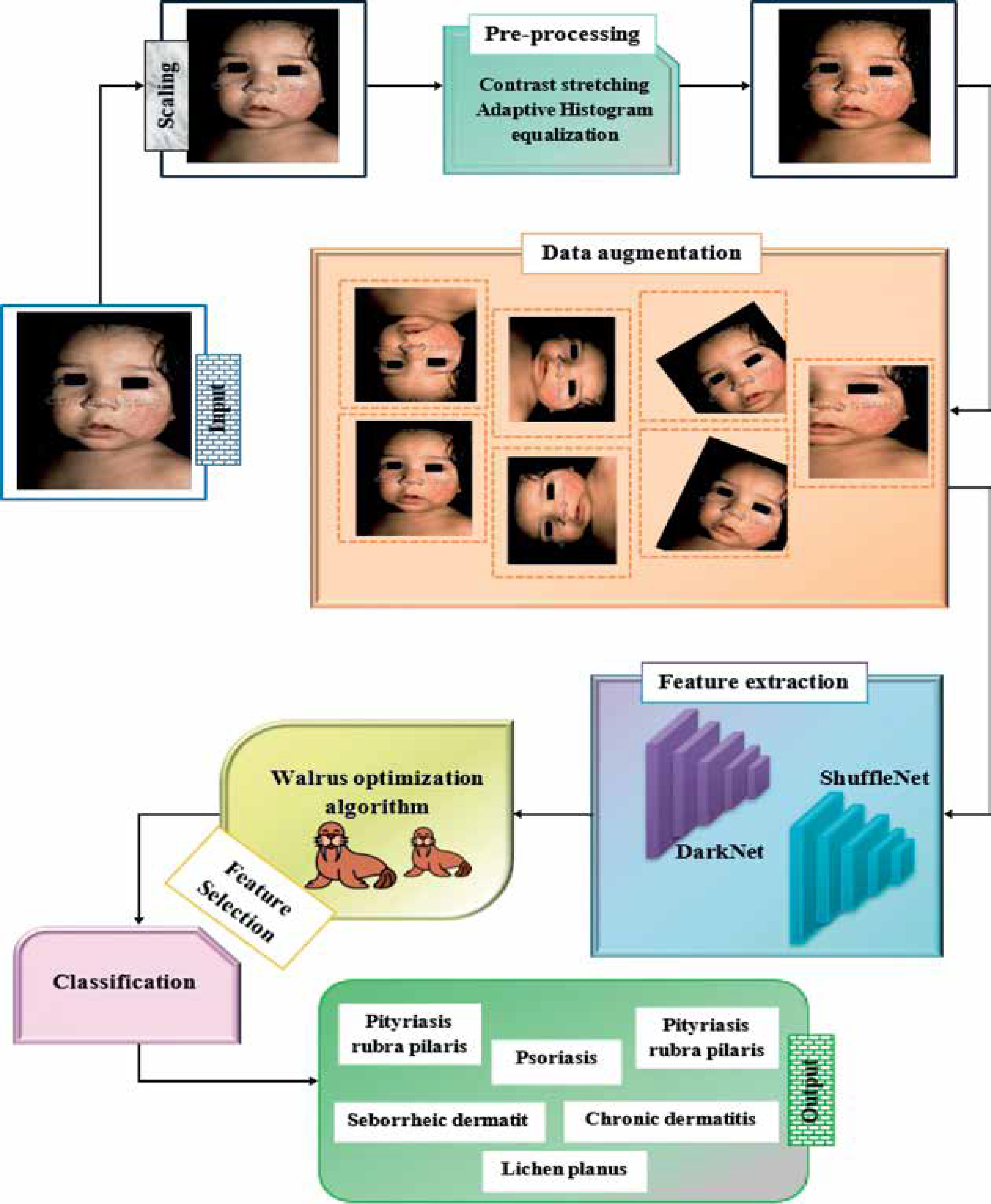
This section introduced a novel Hexa-ESD framework to classify the ESD cases from the available clinical skin dataset. In this model, a Duo-Net is introduced for extracting the spatial features using DarkNet and ShuffleNet. The features are selected using the WalO algorithm to classify the hexa cases of skin diseases. The schematic workflow is presented in Figure 1.
Data description
In this research work, we have created a self-prepared dataset by gathering different clinical skin images from available sources (https://www.kaggle.com/datasets/shubhamgoel27/dermnet). For this preparation, we have collected these images based on the information in the UCI repository [21] (https://archive.ics.uci.edu/dataset/33/dermatology) gathered by Ubeyli and Guler to classify the ESD types. Among the 33 features and predictions, 12 clinical features (e.g., erythema, scaling, itching, Koebner phenomenon, different limits, polygonal papules, and (g) follicular papules) are included. Other factors include (h) involvement of the oral mucosa, (i) involvement of the knees and elbows, (j) involvement of the scalp, (k) family history, and (l) age. There are 366 observations in this dataset that include eight missing values for the “Age” variable [22–26].
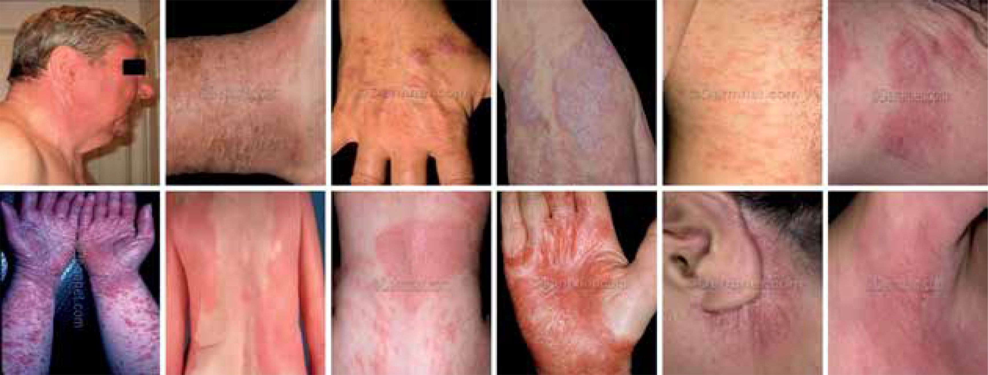
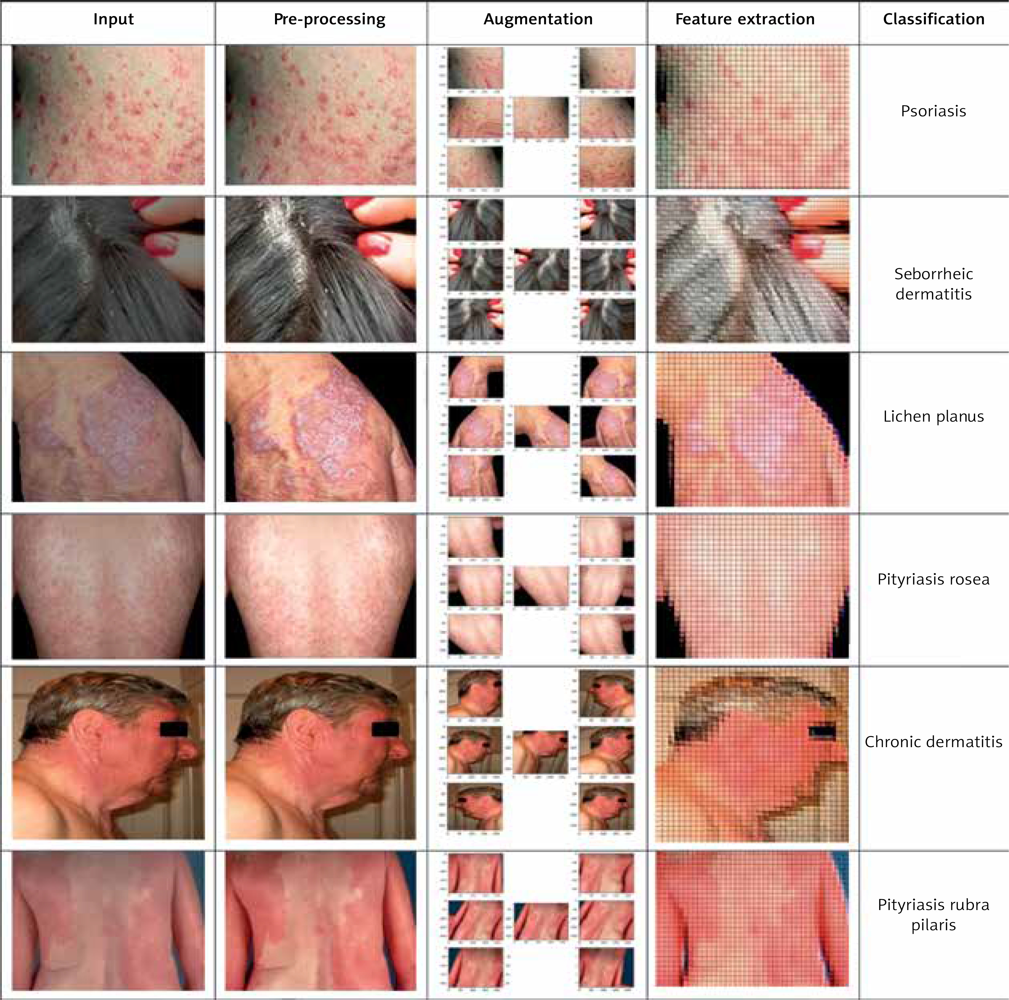
In our self-prepared ESD_DATASET_348, the clinical skin images are manually relabelled from the Kaggle dataset based on the organized classification provided by the UCI repository. This method enhanced the quality of the dataset and preserved uniformity in class definitions. The sample images from our self-prepared dataset are displayed in Figure 2 with hexa different classes of ESD. All the hexa classes are signified due to the 155 images provided by UCI and the 193 images provided by Kaggle as illustrated in Table 1. The distribution shows the class-specific totals by maintaining data sources stable. The target variables are hexa classes and each class includes psoriasis (111 images), seborrheic dermatitis (52 images), lichen planus (71 images), pityriasis rubra pilaris (20 images), chronic dermatitis (46 images), and rosea (48 images).
Data pre-processing
In this denoising phase, every original intensity value is replaced, and the comparison of histograms is conducted through a locally modified contrast-stretching adjustment. The CSAHE is a combination of contrast stretching [27] and adaptive histogram equalization [28] to remove the noise from skin images. The new range is allocated to each pixel by employing a flexible transfer-function derived from the characteristics of the input images. The linear filters that are formed by merging the pixel intensity values of adjacent inputs yield the output pixel values from the input images. This method pursues to increase the contrast between various structures, improve image visualization, and aid in the identification of various ESD cases by applying CSAHE on images. The original level is delivered to every pixel by use of a configurable transfer function that is generated from the attributes of the input images. Assuming that that refers to the input image and that the range of input intensity is calculated.
Where Lmax and Lmin are represented as maximum and minimum intensity values of the input clinical skin image respectively. Now an additional intensity is included for each pixel stated in equation (2)
where qi denotes the adaptive intensity offset added to each pixel, computed based on the local intensity distribution to enhance contrast between structures. The pixel values are modified using the formulas described previously. These values depend on the local image characteristics in which qi is calculated based on the local intensity distribution of the image to enhance contrast between structures.
Here, fj is the adjusted pixel intensity after transformation, Li defines the intensity value of the ith pixel, rj is the scaling factor for the jth pixel, and Qmin and Qmax denote the minimum and maximum gray-level values within the local image region. These pixels are targeted for adjustment according to the conditions in (3). The result is an enhanced image feature and reduced noise in the image. Image manipulation uses histogram equalization to re-distribute pixel intensities for improved contrast. The final resultant image is generated by combining all the sub-images.
Data augmentation
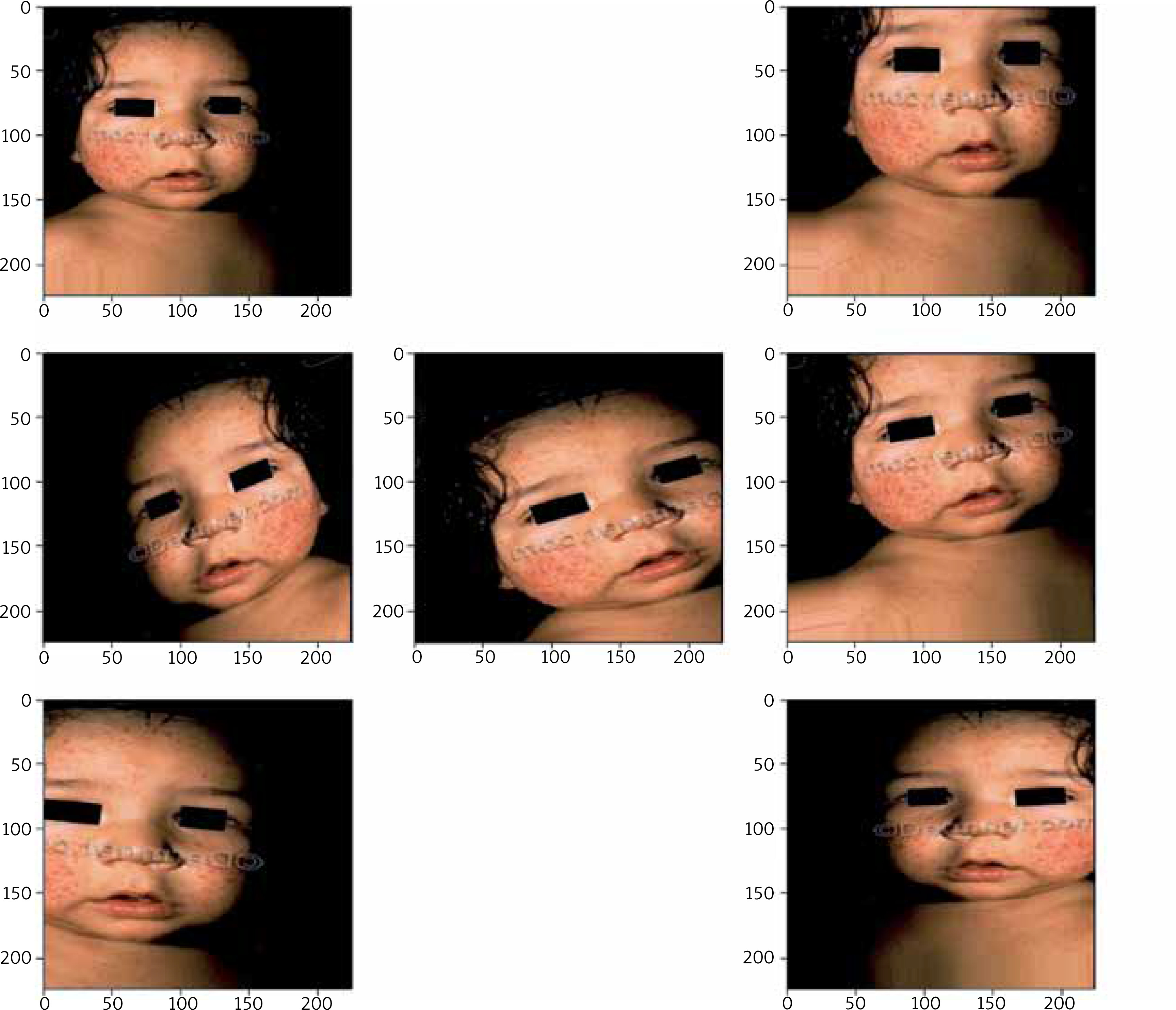
In this phase, various augmentation methods like rotating, zooming, flipping, and rescaling are utilized for increasing the input samples. The sample size was increased using standard augmentation methods such as scaling, flipping, and zooming, introducing more variation to the training set. This allows the model to train on a varied range of clinical skin images, reducing overfitting and improving sensitivity and predictive performance. Through these changes, the training set contains a diverse group of images. The major variations can be incorporated into the training process due to the variety of clinical skin images included in the dataset. Thus, we can lessen overfitting and enhance the sensitivity and predictive abilities of our proposed model. We scaled each image to a fixed 64 × 64 pixel size and extracted RGB values from each image to use as features. The description of the self-prepared dataset before and after augmentation is shown in Table 2. The self-prepared ESD_DATASET_348 is divided into 1120 images for training (80%) and 620 images for testing (20%). The seven different angles of a clinical skin image are shown in Figure 3.
Duo-Net for feature extraction
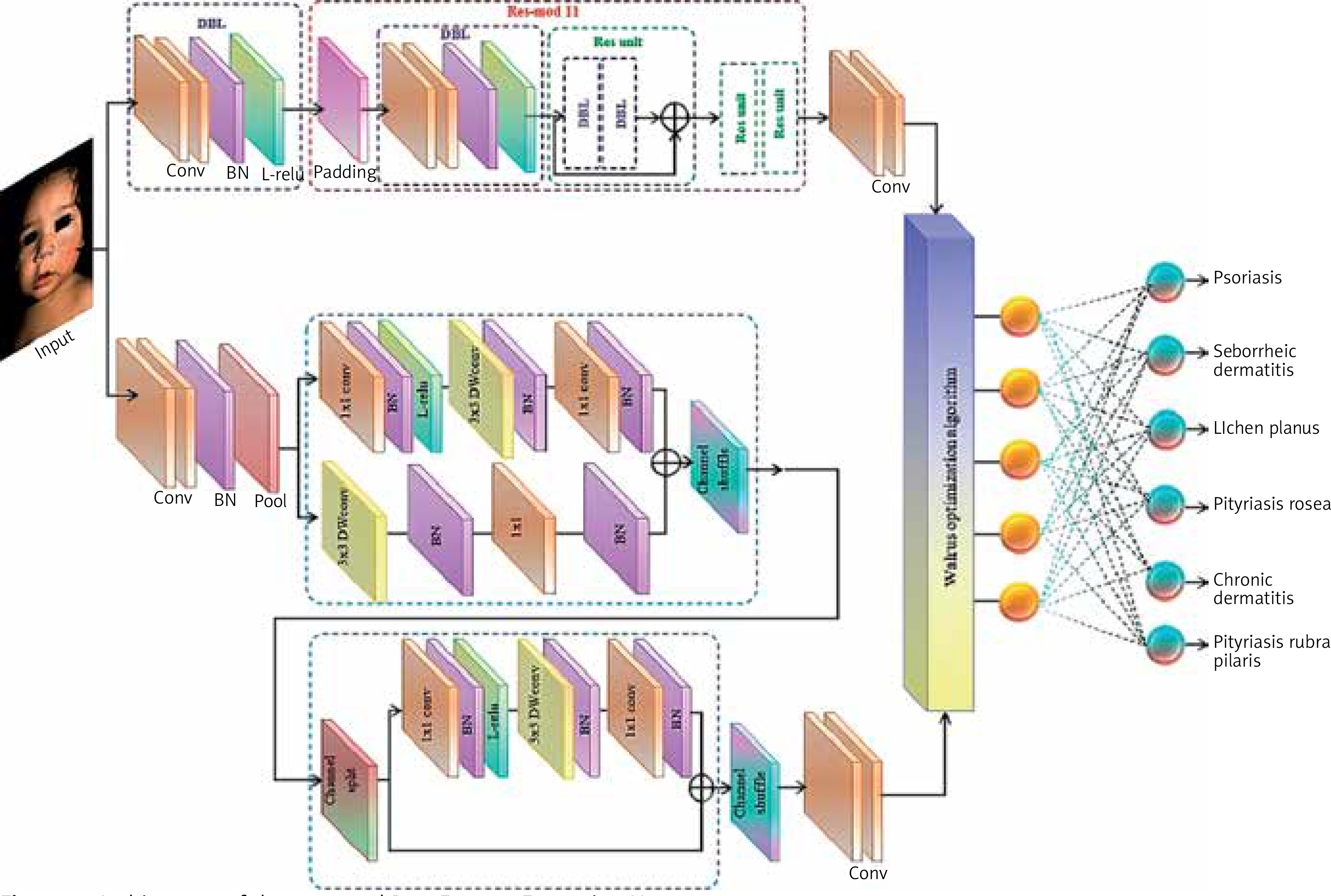
The proposed Duo-feature extraction network is a hybridization of DarkNet and ShuffleNet for extracting the relevant features. The structure of the Duo-feature extraction network is shown in Figure 4.
DarkNet-53
In this phase, DarkNet-53 (DN-53) [26] is employed for extracting relevant features from the input clinical skin images. DN-53 splits the feature maps into two parts and processes each half independently via separate network branches. This network is used in various computer vision tasks for feature extraction. DN-53 consists of 53 convolutional layers organized into multiple blocks. The DN-53 uses a DBL module that comprises a convolution layer of DarkNet (DNconv), batch normalization (BN), and a Leaky-ReLU activation function. The architecture employs skip connections, which allow information to bypass one or more layers and flow through the network more efficiently. This leads to improved data exchange and enhanced feature reuse across different stages of the network. In DN-53, convolution is performed in the convolutional layers, and the architecture has been optimized to merge feature maps from the early stages of the network to the last layers. The convolutional layer is applied to retrieve the vital characteristics from the input data using convolutional filters. Let the input feature map be represented as Iw× Ih× Ic, where Iw, Ih, and Ic denote the width, height, and number of channels respectively.
This correlated portion is made up of “n” residual units (Res-unit) and the residual block (Resblock). A residual unit is then created by connecting two DBL parts. The branch of the first dimension convolves and up-samples the feature map to create new features. The third residual block of DarkNet-53 is then fused with the fourth residual block to enhance feature representation. Finally, the convolutional layer and DBL layer are employed to obtain the feature map with the result. To create new features, the dimension of the feature map is convolved, up-sampled by the second dimension’s branch, and spliced and fused with the third residual block of DN-53. After that, a convolutional layer and a DBL layer are used to generate the final result.
The model applies max-pooling multiple times, adjusting the size of the input windows to build the feature set while using convolutional layers to extract feature maps from images. Initially, input feature maps of varying sizes undergo three convolution steps, followed by max-pooling with various kernel sizes. This approach allows the model to detect and analyse features at different scales and sizes. Max-pooling layers downsampled the spatial dimensions to capture features more effectively. The resulting feature maps represent hierarchical characteristics from the input image, and the final DN-53 model balances speed and accuracy, improving network performance with high efficiency.
ShuffleNet
ShuffleNet [29] is utilized in feature extraction that removes redundant features from the clinical skin images. ShuffleNet downsampling introduces two main changes. Rather than appending the data, first a 3x3 average pooling layer is created with a stride of 2, then use channel cascaded to increase the channel dimension at a low cost. The input is provided as follows:
where I defines input, and Nc indicates the number of channels. Hc and Wc defines the height and width of feature maps. The flops required for ShuffleNet are derived in (5),
where g signifies the number of groups which indicates the number of channels and bottleneck channels M. In equation (4), CM is the product of input channels (C) and bottleneck channels (M) indicating the computation cost of grouped convolutions. The channels were reduced and processed channel-by-channel during ShuffleNet operations. GAP is used in the shuffling phase that the surface features generated by channel-wise data. The spatial dimensions of the input feature map, represented by Hc and Wc are key factors in determining the global average pooled feature vector Z ∈ RNc, which uses global average pooling as its basic aggregation method.
First, a 3x3 convolutional kernel-corresponding single-channel feature maps are generated for each channel. There is no difference in the results of pointwise convolution and ordinary convolution, but significantly less processing is required. The output is passed to leaky ReLU to reduce the non-linearity and gives the value for the threshold that cannot neglect the small changes in the input. The activation function S is determined as,
where δ denotes the Leaky ReLU activation function, and W i, Wj ∈ R represent the learnable weight parameters of the feature extraction layers. Leaky ReLU is used to overcome the difficulties of dying ReLU problems. After the process of concatenation, this network takes feature maps as inputs, which reduces computational costs and increases training capacity.
Feature selection
Feature selection reduces the dimensions of data by choosing the optimal feature group from a high-dimension feature space according to predefined criteria. A feature space also contains redundant, irrelevant, and relevant features. Decreasing the number of features extracted from images and choosing a subset from the available features. A feature selection technique is widely used for both classifying previously unknown important characteristics and removing redundant features that do not contribute to categorization. The process of feature selection is frequently used to eradicate unrelated features to categorize previously unknown traits. The WalO algorithm [30] is a feature selection procedure that chooses the significant features from ShuffleNet and DarkNet based on the natural behaviour of walruses.
In this WalO algorithm, the initial input population is set as 50 walruses with each individual representing a unique feature set. Each solution is defined by 20 variables, corresponding to different features derived from the input. The algorithm iterates through 100 generations, where it refines these solutions by evaluating and selecting the best features. These parameters are typical for balancing exploration and computational cost in feature selection tasks to accurately classify the hexa ESD cases. To determine which features are most pertinent, the retrieved features are fed into the WalO algorithm. The WalO algorithm procedure uses the retrieved features to select the best features. The searcher members of the population used by the population-based metaheuristic WalO algorithm are walruses. Every walrus in the WalO algorithm signifies a possible solution to the optimization problem. The stopping criterion is set as a maximum of 100 generations when the change in the objective function (OF) falls below the consecutive generations which indicates the convergence rate towards an optimal solution. Based on the walrus’s natural activities, the procedure of updating its position in the WalO algorithm is divided into three phases as shown in Figure 5.
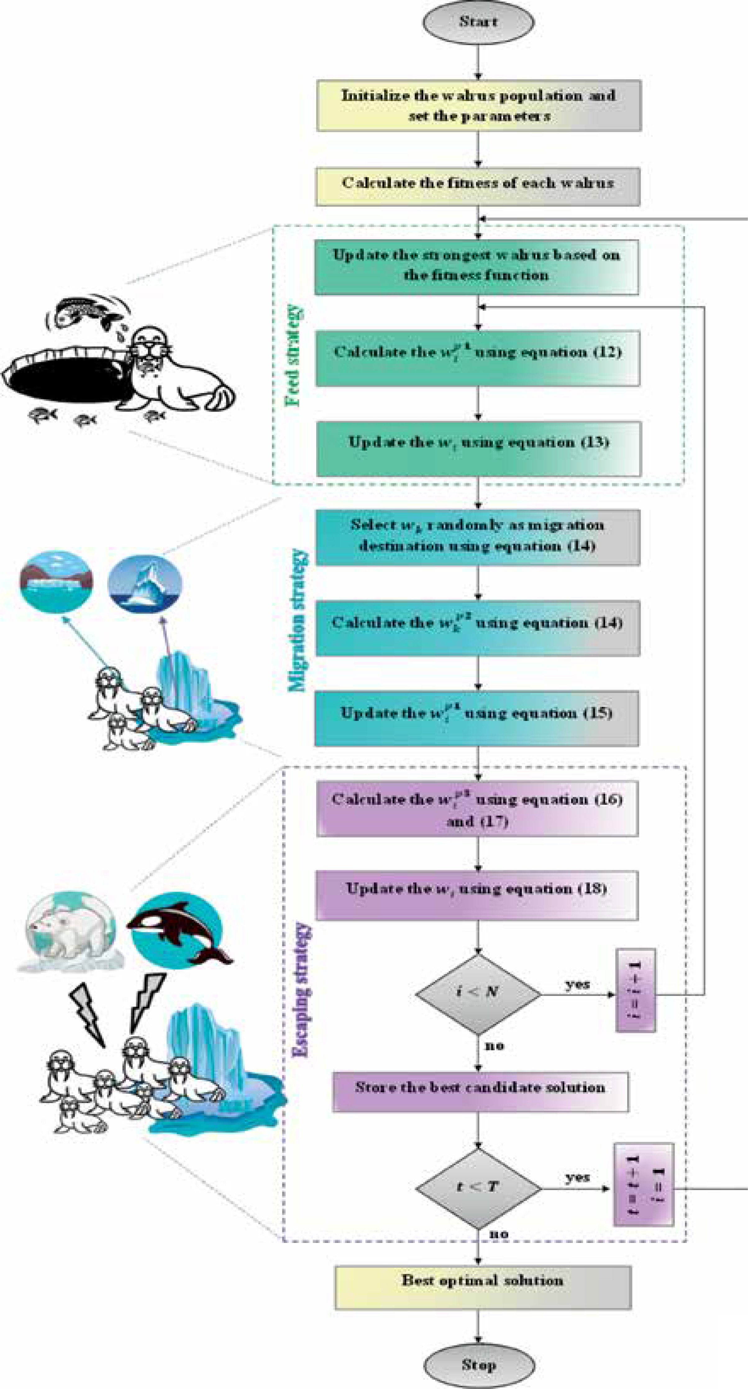
Phase 1. Feeding strategy: Walruses consume about 60 different class of marine animals. It is the strongest walrus in the group with the strongest tusks who lead the others in their hunt for food. There is a correlation between the walrus’ tusk length and the calibre of the OF values of the potential solutions. Thus, the strong walrus in the group is the solution with the highest OF value. In the global search, the WalO algorithm is enhanced by the numerous scanning zones of the search space produced by the walruses.
The exploration strength of the WalO algorithm in global search is enhanced by the walruses’ habitual scanning patterns, which result in diverse scanning areas of the search area. A statistical simulation of walrus position updates is done using (8) and (9), with the most important member of the group serving as guidance. This operation generates a new site for walrus based on equation (8). In equation (9), the new location takes the place of the preceding one if it increases the OF.
where
Phase 2. Migration strategy. Walruses migrate to stony beaches or outcrops when the air warms in the late summer. In the WalO algorithm, migration is used to guide the walruses to areas that are suitable for discovery. Walruses travel to different destinations in distinct regions of the search space according to this model. This results in the generated new place being generated with equation (10). If the OF increases, then this new location takes the position of the walrus.
where
Phase 3. Escaping strategy. Walruses are continually attacked by killer whales and polar bears. Through their strategies to escape and protect themselves from these predators, walruses adopt different postures around their sites. Best-escaping walrus signified the finest feature, and the worst-escaping walrus signified the worst feature. The finest part of the trip is avoiding polar bears and killer whales. There is nothing worse than when killer whales or polar bears kill people. During the feature selection, the worst feature was removed. The following procedure briefly explains this feature selection method. The WalO method simulates this behaviour by creating a new position within the vicinity of each walrus, using (12) and (13).
In this case, equation (14) states that the new location takes over the preceding site if the goal function value is increased.
where
Classification
A random set of features is added after multiplying the input by the feature vectors. DBN with additional categorization is derived from the WalO algorithm, which uses the features acquired from attacking and migrating operations. DBN is a probabilistic generation module made up of several Restricted Boltzmann machines (RBM). The visible and hidden units of the RBMs are connected but not to one another internally, and the hidden units can receive input from the higher-order relationship of the visible units. Energy-based approaches characterize the joint distribution of RBMs as,
where z = ΣvΣh exp (–E(v, h; θ)), the probability of the visible unit being active is
The energy function for RBMs, featuring binary units in both the visible and hidden layers is expressed as follows:
Among the visible and hidden units, wij represents the connection weight between visible unit vi and hidden unit hj, while bi and aj denote the bias terms of the visible and hidden layers respectively. The variables M and N indicate the number of visible and hidden units. The DBN uses the cross-entropy loss function that estimates the variance between the detected prospect distribution and the actual distribution in ESD classification. It assigns higher penalties to incorrect predictions and guides the DBN to improve its accuracy. The cross-entropy loss is calculated as,
where yi is the true class label,
Table 3 illustrates the hyperparameters of the DBN which controls the learning process and overall performance. The learning rate (0.001) defines the step size during gradient updates for ensuring steady learning. Weight decay (0.0001) regularizes the network by reducing overfitting. A batch size of 64 ensures efficient updates by processing data in manageable chunks, while 200 epochs allow sufficient training without overfitting. The dropout rate (0.3) prevents overfitting by randomly deactivating neurons, and weight decay (0.0001) regularizes the DBN to avoid large weight updates. Hidden layers and neurons with 512, 256, and 128 units were chosen to capture relevant features while reducing complexity. During the hyperparameter tuning process, 10% of the training data was reserved for validation. As a result, the efficiency of the proposed Heax/Hexa-ESD was optimized before being tested on the test set. The cross-entropy loss function minimizes the error among detected and actual outputs by guiding the learning process of the DBN in the ESD classification task.
Results and discussion
The experimental arrangement was executed with Matlab-2020b, and the capability of the proposed Hexa-ESD model was evaluated with various efficiency metrics.
Clinical skin images for the input are gathered from the accessible dataset and evaluated using different metrics. In addition to the capabilities of the proposed Hexa-ESD, the comparison provides a thorough explanation and scrutiny of the overall accuracy rate. Additionally, the proposed network is compared with existing DL networks.
Figure 6 portrays the fallouts of the proposed Hexa-ESD framework with the self-prepared images to classify the ESD cases. Besides, the skin images from the collected dataset were denoised by the CSAHE technique to eradicate the unwanted artifacts and augment these images to increase the dataset. The next method was carried out in two steps by segmenting the images by retrieving the relevant features from the denoised images with Duo-feature extraction networks. DBN is applied to categorize the ESD into 6 different cases in terms of the best features.
Competence analysis
The competence of the Hexa-ESD Model was assessed with the network metrics viz., precision (P), F1 score (F1), specificity (S), accuracy (A), and recall (R).
where TP and TN denote the true positives and true negatives of the sample images, respectively, while FP and FN represent the false positives and false negatives of the input images. For the experimental setup, the hexa classes of ESD are defined as “class-0” for psoriasis, “class-1” for seborrheic dermatitis, “class-2” for lichen planus, “class-3” for pityriasis rosea, “class-4” for chronic dermatitis, and “class-5” for pityriasis rubra pilaris. The competence of the Hexa-ESD model for classifying several forms of ESD is tabulated in Table 4 and it is visually shown in Figure 6.
Table 4
Competence valuation of the proposed Hexa-ESD framework
The Hexa-ESD framework classified the six different ESD classes from class-0 to class-5 as shown in Figure 7. The proposed Hexa-ESD is measured in terms of A, P, R, S, and F1 respectively. The proposed Hexa-ESD model reaches A of 97.69%. Also, the proposed Hexa-ESD method displays an overall S of 96.63%, P of 97.06%, R of 97.54%, and an F1 of 98.35% respectively.
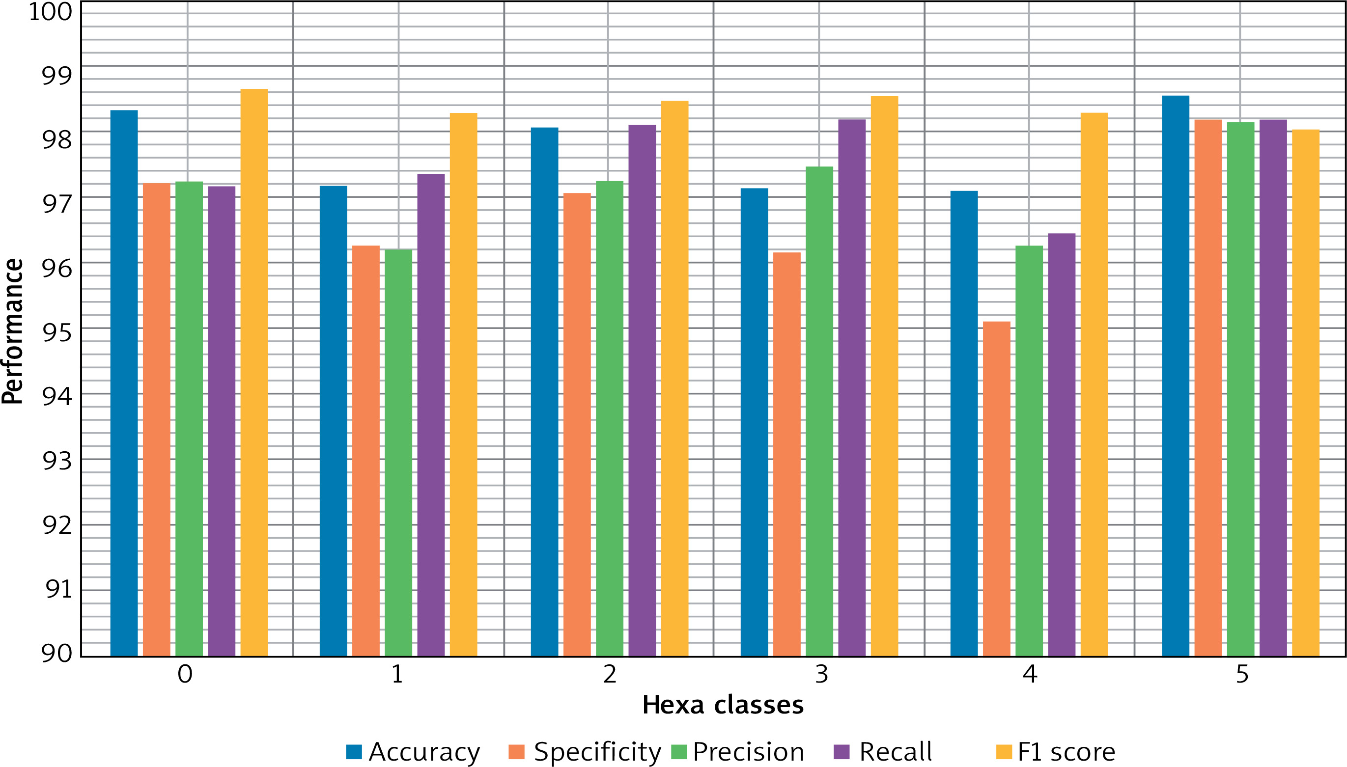
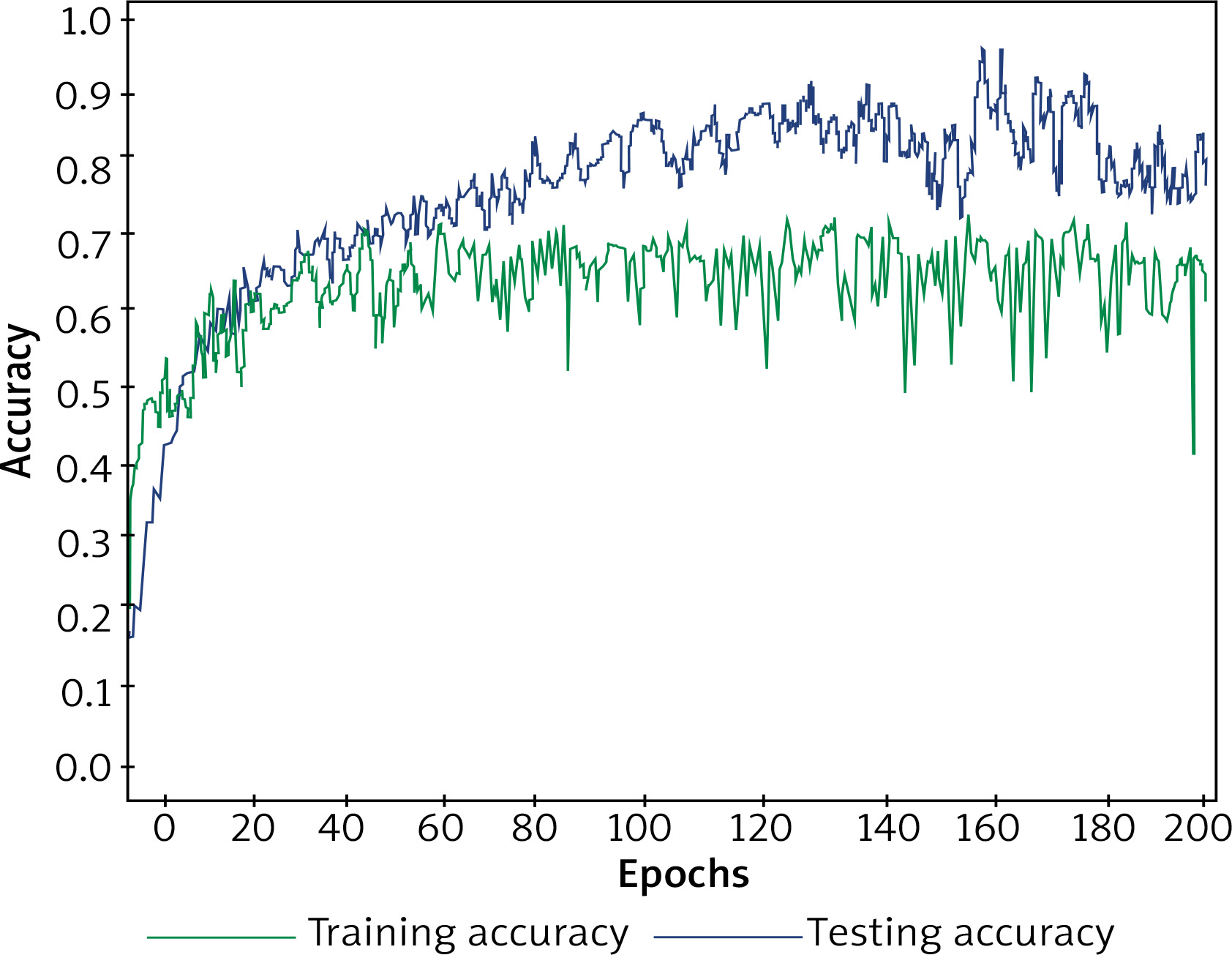
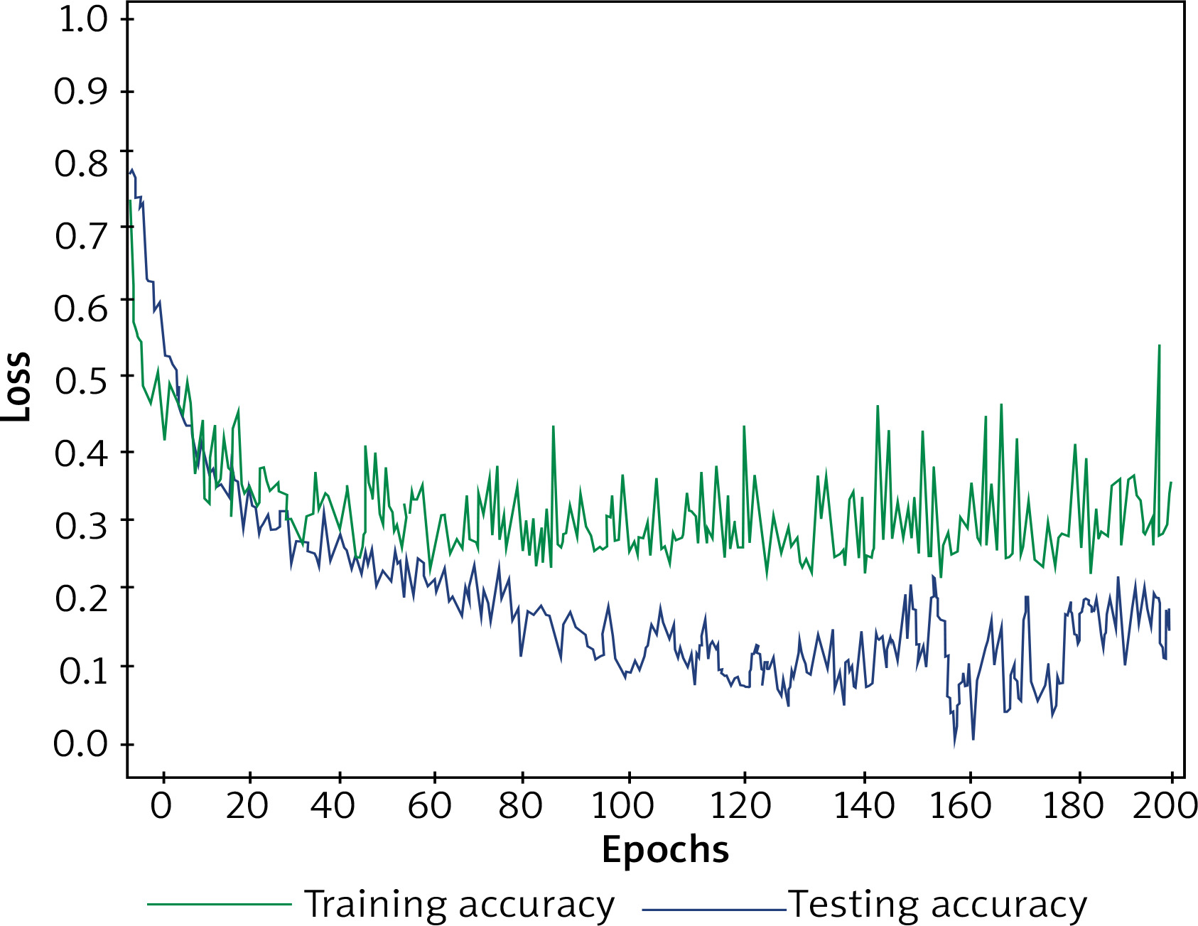
Figure 8 depicts the accuracy curve, showcasing the accuracy on the x-axis against the number of epochs on the y-axis. The accuracy of the Hexa-ESD increases with more training epochs are illustrated in Figure 9, where the loss decreases as the epochs progress. In this study, we aim to determine how many training epochs are best for obtaining high testing accuracy. The results indicate that after 200 epochs, the Hexa-ESD framework attains a notable classification accuracy of 97.69%, with a low error rate.
Moreover, we evaluated the performance of the proposed Hexa-ESD using 3-fold and 5-fold cross-validation to ensure the robustness and reliability of the Hexa-ESD framework. The dataset was split into respective folds, and the results were averaged across all runs with two different cross-validations (CV) as illustrated in Table 5.
Table 5
Cross-validation outcomes of the proposed model
| Metric | 3-fold CV | 5-fold CV |
|---|---|---|
| Accuracy (A) | 96.8% | 97.1% |
| Precision (P) | 96.4% | 96.8% |
| Recall (R) | 96.6% | 96.9% |
| F1-score (F1) | 96.5% | 97.0% |
| Specificity (S) | 96.3% | 96.7% |
In addition, the 3-fold and 5-fold CV results support the robustness of the Hexa-ESD framework. In the 3-fold and 5-fold CV, the dataset is separated into 577 and 328 images for testing, 1173 and 1412 images for training. The fallouts of a 5-fold CV indicate that more folds can lower bias and variability and produce more reliable performance results. Those findings confirm that the suggested framework generalizes effectively across different data partitions, which is consistent with the previously reported accuracy of 97.69% based on a single 80-20 split of the dataset.
Comparative analysis
The predicted performance of each DL network was measured to confirm that the proposed Hexa-ESD framework achieves a high level of accuracy. Competency evaluations compared the Hexa-ESD framework to four DL networks, including CNN and RNN methods. The Hexa-ESD framework demonstrated superior accuracy, achieving a rate of 97.69%, outperforming traditional DL networks. Various parameters were used to evaluate the efficacy of each DL network during the assessment.
To maximize classification accuracy for ESD instances, a comparison of various conventional models was performed, as detailed in Table 6. Figure 10 presents a visual analysis between the Hexa-ESD framework and these conventional networks. Notably, models like AlexNet, DenseNet, and LeNet demonstrate lower accuracy compared to ShuffleNet and DarkNet. The proposed ShuffleNet increases the accuracy by 6.48%, 5.35%, and 2.21% better than AlexNet, DenseNet and LeNet respectively. Furthermore, the proposed DarkNet increases the accuracy by 10.08%, 9.0%, and 5.96% better than AlexNet, DenseNet and LeNet respectively. From this analysis, the proposed Hexa-ESD framework achieves a better accuracy of 97.69% due to the combination of ShuffleNet and DarkNet models.
Table 6
Comparison among conventional networks
| Conventional networks | S | P | R | F1 | A |
|---|---|---|---|---|---|
| AlexNet [22] | 88.52 | 87.19 | 87.16 | 88.21 | 88.15 |
| DenseNet [23] | 86.17 | 85.42 | 85.32 | 87.03 | 89.21 |
| LeNet [24] | 90.04 | 89.14 | 88.05 | 89.14 | 92.17 |
| ShuffleNet [25] | 98.11 | 93.05 | 94.82 | 94.51 | 94.26 |
| DarkNet [26] | 97.28 | 97.04 | 96.80 | 96.28 | 98.04 |
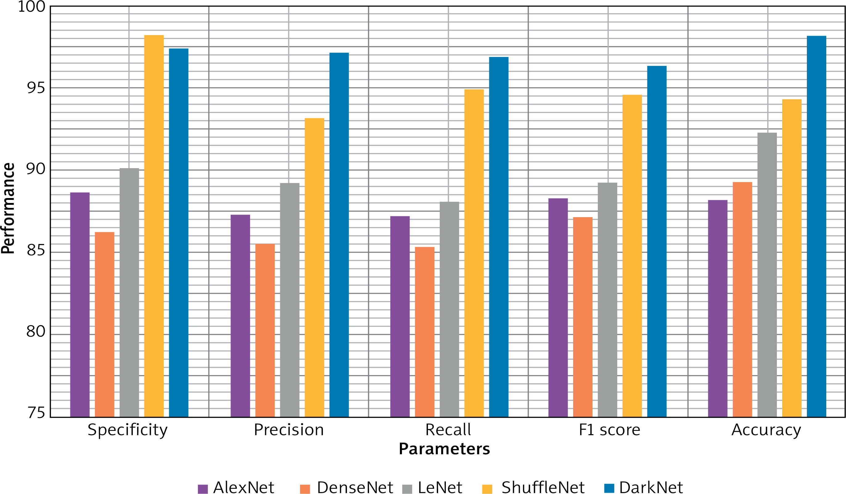
Table 7 compares the parameters of different neural networks for ESD detection. The proposed DBN model achieves the highest accuracy (97.69%) and specificity (96.63%), outperforming DNN, CNN, RNN, and ANN across all metrics. The DBN also attains high precision (97.06%), recall (97.54%), and F1 score (98.35%) for indicating superior classification performance compared to the other models. CNN shows strong performance with 97.15% accuracy, while ANN has the lowest accuracy at 93.54%. The DBN increases the average accuracy range by 1.65%, 0.55%, 2.27% and 4.24% better than DNN, CNN, RNN and ANN respectively. The DBN model demonstrates a significant improvement in detecting ESD cases compared to other existing classifiers.
Table 7
Comparison of existing classification networks
| Networks | A | P | R | S | F1 |
|---|---|---|---|---|---|
| DNN | 96.07 | 95.25 | 95.28 | 96.03 | 95.23 |
| CNN | 97.15 | 95.04 | 95.63 | 95.25 | 96.35 |
| RNN | 95.47 | 94.28 | 94.87 | 95.04 | 95.04 |
| ANN | 93.54 | 92.12 | 93.24 | 92.25 | 93.18 |
| DBN | 97.69 | 97.06 | 97.54 | 96.63 | 98.35 |
As shown in Table 8, the testing process measured the time taken to process an input signal from the dataset to assess the accuracy of various approaches. The performance of previous methods was compared using specific criteria to ensure correct classification accuracy. The proposed Hexa-ESD framework increases the overall accuracy of 3.26%, 1.93% and 18.21% for ReliefF Algorithm [17], Extreme Gradient Boosting [18] and Enhanced Pipeline Feature Selection (EPFS) Algorithm [19] respectively. However, the prior techniques have not reached the best accuracy range when compared to the Hexa-ESD framework.
Conclusions
This work introduces a Hexa-ESD model to efficiently categorize the clinical skin images into various skin diseases. The DL-based DarkNet and ShuffleNet were employed to retrieve the spatial features from the pre-processed images. Then, these retrieved features were fed into the WalO algorithm by dealing with complex non-linear problems for selecting the best features. These selected features were fused for classification using a fully connected layer to detect the hexa ESD cases. The efficiency of the Hexa-ESD was assessed with some metrics like S, P, R, A and F1. From this analysis, the Hexa-ESD framework achieves a better accuracy of 97.69% due to the combination of ShuffleNet and DarkNet models. The proposed ShuffleNet rises the accurateness/accuracy in 6.48%, 2.21% and 5.35% better than AlexNet, LeNet and DenseNet respectively. Furthermore, the proposed DarkNet increases the accuracy by 10.08%, 9.0%, and 5.96% better than AlexNet, LeNet and DenseNet respectively. The Hexa-ESD framework increases the overall accuracy by 3.26%, 1.93% and 18.21% for ReliefF Algorithm, XGBoosting and EPFS algorithm respectively. The result of the Hexa-ESD framework attains precise results compared with the existing networks. The inclusion of hair in rare cases and conditions deduces the categorization accuracy of the proposed Hexa-ESD to recognize a wide range of skin disorders. In the future, we will develop a model that can provide accurate diagnosis in the presence of hairs through advanced DL models. Additionally, we plan to collaborate with domain experts to construct or use more rigorously labelled datasets to mitigate dataset inconsistencies.