
Purpose
Current commercially available treatment planning systems (TPS) for high-dose-rate (HDR) brachytherapy, such as Oncentra Prostate (OcP) and Oncentra Brachy (OcB) (Elekta, Veenendaal, The Netherlands), offer different plan generation tools that are implemented on central processing unit (CPU) architecture. For instance, forward planning techniques, such as graphical optimization (GrO) [1] or efficient inverse planning algorithms, i.e., inverse planning simulated annealing (IPSA) [2], hybrid inverse planning optimization (HIPO) [3, 4], and dose-volume histogram-based optimization (DVHO) [5, 6], can be used to optimize dwell times in OcP. In addition to dose-volume histogram (DVH) curves and 3D dose computations, these optimization algorithms require around 10-20 seconds to generate a single treatment plan on a commercially available clinical workstation [6]. While TPS provide sufficient computing power for most planning tasks in HDR brachytherapy, there are certain situations, in which more computational power may be useful [7]. For instance, repeatedly optimizing treatment plans with IPSA or HIPO with various trade-offs to explore Pareto surfaces as in multi-criteria optimization (MCO), can be time-consuming (few hours of computational resources) [8, 9]. Given that trade-offs are patient-specific due to different diagnosis and patient geometry, manually tweaking the objective function (with IPSA or HIPO) and/or dwell times (with GrO) to explore the solution space as it is routinely done in clinic, can be cumbersome, time-consuming, and can lead to sub-optimal plans of patients [1, 10].
To overcome the computational burden of calculating multiple plans, different MCO approaches were investigated. In Cui et al., regression models combined with parallel plan computation on CPU were designed to narrow down the clinically relevant solution space, and to reduce the planning time [8, 11]. In Deufel et al., a library of Pareto optimal plan was constructed and used to approximate different trade-offs by using near real-time (0.1 s) interpolation techniques [12]. Another approach was proposed to combine graphics processing units (GPU) with MCO algorithms to generate patient-specific sets of Pareto-optimal plans (hundreds to thousands plans) in a clinically acceptable time-frame (within 1 minute) [13, 14]. Consequently, MCO has great potentials to improve the plan quality as well as planning efficiency in the clinic [8, 11, 15-17].
In our previous study, the impact of combining our graphics processing unit (GPU)-based multi-criteria optimization (gMCO) algorithm [13], with an interactive graphical user interface (gMCO-GUI) for HDR brachytherapy [18], was evaluated. With gMCO, it is expected that the planning tasks will be shifted from iterative plan tuning to patient-specific plan navigation and selection. Motivated by the computational efficiency offered by GPUs and MCO algorithms for HDR brachytherapy planning, this study takes a step further by rigorously commissioning and validating our MCO workflow against the standard clinical workflow. More specifically, since it is well-known that the dosimetry (e.g., dosimetric indices) differs from one TPS to another [19-21] as a consequence of numerical parameters [22], this work ensures that the dosimetry of gMCO plans agrees with the dosimetry calculated by two widely used and clinically validated TPSs. This will ensure that the proposed MCO workflow can be safely integrated in the clinic.
Material and methods
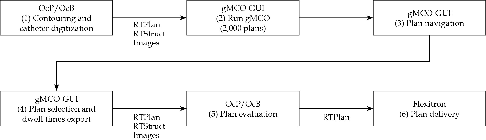
gMCO algorithm was commissioned against the clinically validated OcP v. 4.2.2 and OcB v. 4.6.0 (Elekta, Veenendaal, The Netherlands) TPSs. Main steps of the proposed MCO workflow are depicted in Figure 1. This study mainly focused on steps (4)-(6) since it is of crucial importance for the clinic that the proposed MCO workflow is compatible and in agreement with a clinically approved TPSs. In other words, gMCO optimizer and gMCO-GUI were used for the treatment plans generation in steps (2)-(3); OcP and OcB optimizers were not used, as OcP and OcB were only applied for plan evaluation (DVH, 3D dose, and isodose) in step (5). Mimic parameters were further introduced to ensure that the dosimetry of gMCO plans displayed in gMCO-GUI matched the dosimetry of OcP or OcB based on recommended threshold criteria.
gMCO algorithm
gMCO algorithm was implemented on GPU architecture with the following computational features: TG43 line source formalism [23], limited-memory Broyden–Fletcher–Goldfarb–Shanno optimizer (gL-BFGS), DVH curves, and 3D dose computations. Hence, gMCO allows the generation of 1,000 Pareto-optimal treatment plans with various trade-offs within 10 sec [13]. gMCO algorithm was compiled using CUDA v. 11.1 and MSVC compiler (Microsoft Visual Studio 2019 v. 16.7.4) on a Windows 10 station. The computations with gMCO algorithm were executed on an Intel (R) Core (TM) i9-10920X CPU (128 Go and 24 cores @ 3.5 GHz) and an NVIDIA GeForce RTX 2080-Ti GPU (11 GB and 4352 CUDA cores).
gMCO-GUI
gMCO-GUI (Figure S1 in Supplementary Material) was implemented to allow the planner to explore patient-specific trade-offs in real-time by interactive navigation through gMCO-generated set of Pareto-optimal plans [18]. Hence, gMCO-GUI displays the dosimetric indices, 3D dose distribution, and DVH curves in real-time during plan navigation [18]. In gMCO-GUI, plan navigation is done by using interactive navigation and constraint sliders [18].
MCO-based re-planning
Forty HDR brachytherapy prostate cancer patients (20 cases planned on ultrasound [US] with OcP and 20 cases planned on computed tomography [CT] with OcB) were retrospectively re-planned with gMCO algorithm. For each case, the prescription was to deliver 15 Gy in a single fraction as a boost to external beam radiotherapy (EBRT). The target, bladder, rectum, and urethra structures were delineated from the images, with a slice thickness of 0.5 mm with OcP (US images) and 2 mm with OcB (CT images). Patients were selected to cover a wide range of prostate volumes from our database of HDR brachytherapy prostates. Information on patients’ statistics can be found in Table 1.
Table 1
Patient cohort statistics for HDR brachytherapy prostate cases, with ultrasound (US)-based and computed tomography (CT)-based planning with gMCO. The values indicate the median and the range in parenthesis
Each case was re-planned with gMCO algorithm by generating 2,000 Pareto-optimal plans. For the 20 US cases, a single treatment plan was chosen by two physicists in gMCO plans bank. The physicists used gMCO-GUI plan navigation tools to find the most suitable plan for each patient. For the 20 CT cases, the plan with the highest target coverage while meeting clinical criteria (i.e., the first planned displayed in gMCO-GUI) was selected in gMCO plans bank [18]. The chosen plans were exported as DICOM-RTPLAN format by saving optimized dwell positions and dwell times. gMCO plans were imported back into OcP (US cases) and OcB (CT cases) to calculate final dosimetry of gMCO plans.
TG43 calculations
In OcP, the TG43 line source formalism is directly used for dose-rate calculations by linear interpolation of radial dose function table and bilinear interpolation of anisotropy function table. This formulation was implemented on GPU architecture in gMCO. For clarity, this TG43 implementation is referred to as ‘gMCO/mimic-OcP’.
In OcB, an along-away table (y-z plane origin at active center of the source) is pre-calculated and used with bilinear interpolation during brachy planning step, based on the TG43 line source formalism, with a small grid spacing (typically 1 mm). This approach was also implemented on GPU architecture in gMCO, with a grid-spacing of 1 mm. Cut-off dose rate was set to 85.6 cGy/hU as in OcB. For clarity, this TG43 implementation is referred to as ‘gMCO/mimic-OcB’.
Computational settings (including the ones for volume, DVH curves, and 3D dose calculations in the following sections) used in gMCO, OcP, and OcB are summarized in Table 2. To validate the GPU-based TG43 implementation in gMCO, dose-rate of flexisource was calculated and compared with consensus data [24]. Accuracy of the calculated dose rates was assessed following the TG-43 report, in which deviations within 2% are acceptable for commissioning of TPSs [23, 24].
Table 2
Computational settings used in gMCO, OcP, and OcB. Mimic parameters used in gMCO are highlighted with bold characters
Volume computations
Random sampling point method, as described in OcP reference manual [25, 26], was implemented in gMCO. For each structure, assuming a delineation of structures in the axial plane, a bounding box containing the structure’s contour plus 1 cm margin in each direction was created to randomly sample dose calculation points via a uniform random distribution (using the C++ linear congruential engine, which has a period of 4.295 × 10⁹). For each dose calculation point, three random coordinates were generated within the bounding box (one for each axis), the closest 2D axial structure contour to the point was found (using the z coordinate), and finally the dose calculation point was classified as within this 2D contour, or not using the point in polygon algorithm [27]. This process was repeated until a user defined number of dose calculation points was achieved in the structure. The volume of structures was obtained by multiplying the box volume with the fraction of points included in the structures and the total number of points specified in the bounding box. The top and bottom slices of the structures were considered as the structures’ extent in the z-axis.
As recommended by Nelms et al. [21], analytical shapes were used as the ground truth to validate the accuracy of dose point sampling algorithm. In this study, three spheres (radius of 0.5, 2, and 3 cm) and two cylinders (radius of 0.5 and 2 cm, and height of 4 cm) with 1 mm slice thickness (along the axial plane) were used. 50,000 random sampling points per shape were sampled with gMCO and OcP, while 200,000 random sampling points per shape were sampled with OcB. These numbers of sampling points were the maximum allowed in TPSs applied as baselines (thus yielding the highest numerical accuracy), and were also used for DVH calculations.
DVH computations
Regarding DVH computations, the urethra volume was part of the prostate volume. For the US cases planned with OcP, the slice thickness of the contours was directly given by the US images slice thickness (0.5 mm). Since dose-rate at dose points close to the source was unknown with OcP, a cut-off dose rate of 1 cGy/hU was empirically set (by trial and error) and used in gMCO when a dose point was inside the source (modelized by a cylinder centered at the source center with r = 1 mm and h = 4.8 mm) to mimic OcP. For the CT cases planned with OcB, the slice thickness of the contours was initially 2 mm (slice thickness of the CT images) and re-sliced with a slice thickness of 1 mm, using interpolation method described in van der Meer et al. [22], which is similar to the method described in OcB. Note that the inter-slicer interpolation was treated as a mimic parameter when calculating DVH curves to mimic OcB. Details of numerical parameters used for the DVH curve computations are included in Table 2.
To quantify the agreement in volume and dose of DVH curves, two approaches were investigated with OcP and OcB as the reference. 1) The difference of 9 key dosimetric criteria calculated from DVH curves were reported. 2) The DVH curves (volume expressed in cc) of each structure were compared using 1D γ analysis (ΔD/ΔV) as described by Ebert et al. [28]. The γ analysis was performed by using γ module of pyMedPhys v. 0.37.1 library [29], which implements a method described by Wendling et al. [30]. In the γ module, dose criterion (ΔD; analog to the ‘distance’ criteria in the γ module) was fixed to 1% of the prescribed dose (ΔD = 0.15 Gy), and volume criterion (ΔV; analog to the ‘dose’ criterion in the γ module) varied from 1% with 1% increment until all the bins passed the γ test (γ≤ 1) for all cases. Global normalization was fixed to the volume of structure calculated by OcP/OcB.
Mitigating the impact of statistical uncertainties on DVH indices
In van der Meer et al., it was well characterized that the random sampling point yields DVH indices, with statistical uncertainties that are dependent on the number of sampling points, or point density [22]. Since gMCO and OcP/OcB implement this method, it was expected that DVH indices would change value according to these uncertainties when calculating plans back-and-forth. This might be problematic for DVH indices close to dosimetric criteria limit. To mitigate this effect and to illustrate the clinical impact, a statistical safety margin was simulated for the bladder V75 and rectum V75, based on standard deviation (σ) of distributions, by comparing dosimetric results obtained with V75 < [1.0 – σ] cc vs. V75 < 1.0 cc (as used to originally generate the plans). The seed of random generator in gMCO was changed 100 times for different number of sampling points (5,000, 10,000, 20,000, 50,000, and 100,000) to estimate the standard deviation of distribution for each number.
Isodose lines and 3D dose computations
For the 3D dose calculations, 1 × 1 × 1 mm3 voxels were used with 1 cm margin around target extents in gMCO. These settings were chosen to balance computational efficiency and memory consumption with accurate resolution of the 3D dose for the isodose lines display in gMCO-GUI. Moreover, the 1 cm margin was sufficient for the visualization of relevant isodose lines (75%, 100%, 125%, and 150%) and OARs displayed in gMCO-GUI. In gMCO-GUI, isodose lines were calculated using a module contour of matplotlib python library; this module implements the marching squares algorithm. In OcP, the 3D dose was calculated with 2 cm margin around the active sources, and voxel size was automatically adjusted depending on the volume (≈ 1 × 1 × 1 mm3). For OcB, the voxel size was 1 × 1 × 1 mm3, and the matrix size was determined with a 2 cm extent around the implant.
In a first step, the validation of displayed isodose lines (placement and shape) in gMCO-GUI was conducted. To this end, the OcB 3D dose was exported as DICOM RTDOSE file format, and the coordinates of the isodose lines calculated by OcB were exported as DICOM RTSTRUCT file format. The isodose lines were re-calculated with gMCO-GUI from OcB exported RTDOSE. The displacement between gMCO-GUI and OcB calculated isodose lines was calculated using 95th percentile undirected/bidirectional boundary Hausdorff distance [31] (referred to as the 95% HD in this study). OcB was solely used for this analysis since, to the best of our knowledge, the isodose lines cannot be converted to RTSTRUCT with OcP. In a second step, the validation of the 3D dose calculated by gMCO was conducted as follows. The isodose lines calculated by gMCO-GUI from the gMCO 3D dose and OcP/OcB 3D dose (exported as RTDOSE) were compared using dice coefficient and 95% HD. In addition, 3D γ analysis [32] was used. For the γ analysis, global normalization was set to the prescribed dose (15 Gy), the minimum dose was set to 10%, and the maximum dose was set to 400%. The thresholds were set to ΔD/Δd = 1%/1 mm for dose (ΔD) and distance (Δd) criteria. The fraction of γ values passing the dose and distance criteria (γ≤ 1 with 1%/1 mm) was reported.
Mimic parameters ON vs. OFF
It should be noted that the gMCO plans were generated with the mimic parameters ON (bold parameters in Table 2) to be representative of clinical usage. The dose of gMCO plans were also re-calculated with the mimic parameters OFF to characterize the impact of mimic parameters. Mimic parameters OFF means that the modifications implemented from Table 2 are inactive; for instance, the dose rate cut-off for OcP and OcB as well as TG43 along-away table and inter-slice interpolation for OcB.
Threshold criterion
Regarding the commissioning of TPSs, TG-53 report [33] does not provide any tolerances and acceptable deviations for the volume, DVH curves, and 3D dose distributions. From previous studies on TPS comparisons, deviations between 1% and 10% were observed in volume or dosimetric indices [19-21]. Furthermore, changes of up to 9.8% in dosimetric indices can be obtained by changing numerical parameters alone [22]. Following the recommendations of Nelm et al., 2% was used as a baseline to assess acceptable deviations for volume and DVH curves [21]. Regarding the accuracy of isodose lines placement, the voxel size resolution of 1 mm was applied as a baseline.
Results
TG43 calculations
Raw dose-rate values calculated by gMCO and raw dose-rate values of the consensus data are presented in Table S1 and Table S2 in Supplementary Material, respectively. Relative differences in dose-rate values are shown in Table S3 in Supplementary Material. Overall, the relative differences in dose rates calculated by gMCO and the TG43 consensus data of flexisource ranged from –0.3% and 0.4%.
Volume calculations
The results of the calculated volumes of three spheres with different radius and two cylinders with different radius are demonstrated in Table 3. Compared with theoretical volumes, the relative differences between –2.9% and 0.1%, –3.3% and –0.3%, and –6.4% and –0.2% were obtained with gMCO, OcP, and OcB, respectively. When comparing structures’ volume between gMCO and OcP/OcB for all cases, the median relative differences were within ±1% (see Figure S2 in Supplementary Material).
Table 3
Volumes calculated with gMCO, OcP, and OcB for three spheres with different radius and two cylinders with different radius and fixed height. Volumes in bold indicate the value the closest to the ground truth volume
DVH computations
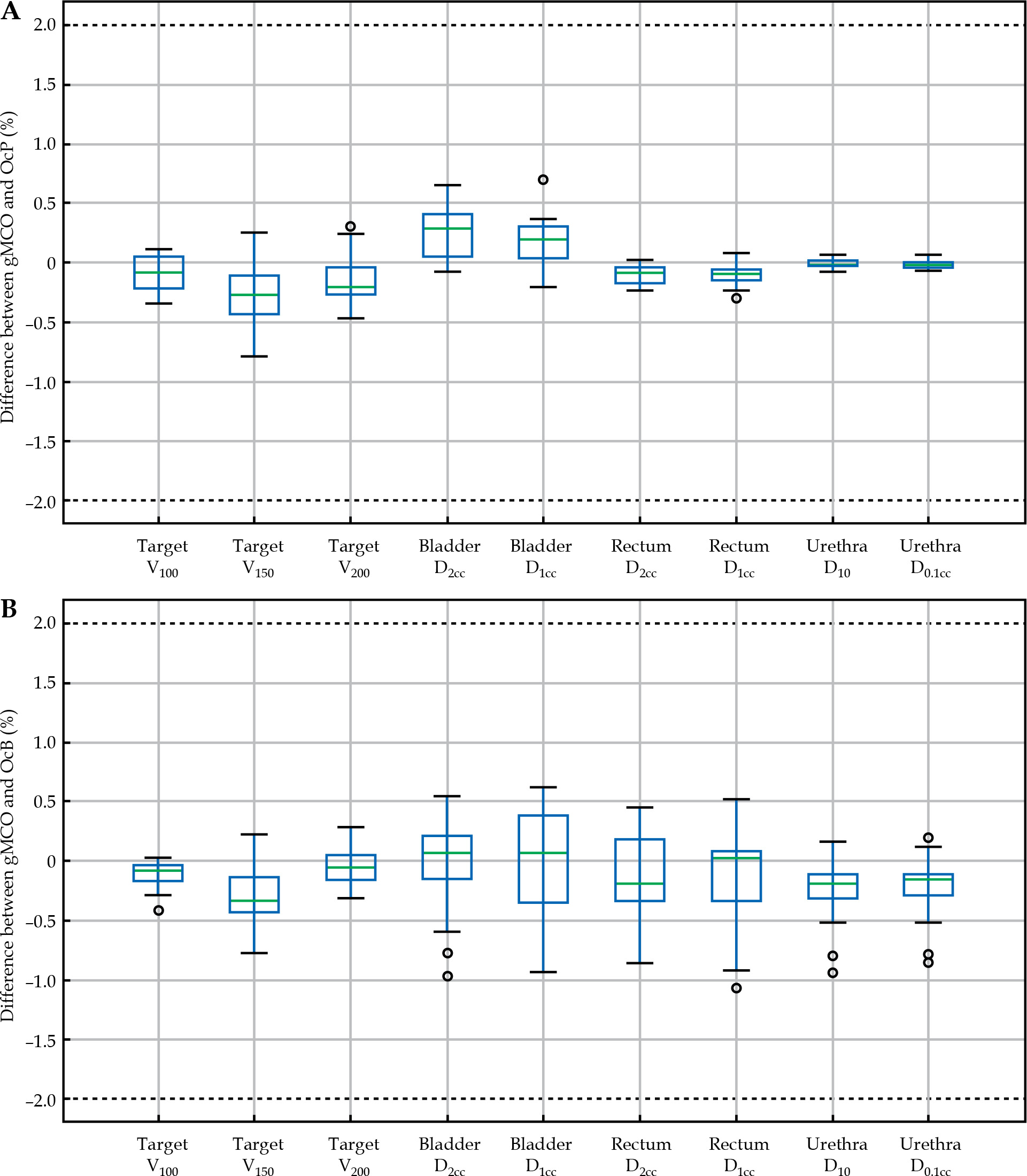
The differences between gMCO and OcP, and gMCO and OcB are depicted in Figure 2 for 9 dosimetric indices with the mimic parameters ON (Table 2). The differences with the mimic parameters OFF in gMCO are included in Figure S3 in Supplementary Material section. As seen in the panels of Figure 2, the differences between gMCO and OcP calculated dosimetric indices values were within ±1% and within ±1.2% compared with OcB. Although not shown in Figure 2, the mean (±SD) differences between the bladder V75 and rectum V75 was 0.01 ±0.01 cc and 0.02 ±0.02 cc (gMCO vs. OcP), and was 0.00 ±0.06 cc and 0.01 ±0.04 cc (gMCO vs. OcB), with a maximum deviation of 0.13 cc (from 0.96 cc to 1.09 cc in the bladder V75).
Fig. 2
Difference between gMCO and A) OcP and B) OcB calculated dosimetric indices. Values of volume dosimetric indices (V) were calculated in fraction (%) of structure volume. Values of dose dosimetric indices (D) were calculated in fraction (%) of the prescribed dose. Mimic parameters were turned ON in gMCO
The top left panel of Figure 3 illustrates the normalized DVH curves calculated by gMCO with OcP-mimic parameters ON compared with OcP for a random case, and the top right panel illustrates the corresponding γ values with 1%/2% thresholds. Bottom panels of Figure 3 illustrate the same curves but with gMCO with the OcB-mimic parameters ON compared with OcB for a random case. The DVH curves obtained the mimic parameters OFF in gMCO for these two cases are depicted in Figure S4 in Supplementary Material section.
Fig. 3
Comparison of DVH curves (left panels) calculated with gMCO compared with OcP (A) and OcB (B) DVH curves for one random case. Right panels illustrate the corresponding γ values with 1%/2% thresholds when comparing DVH curves (volumes in cc). Global normalization (GN) for the γ test was set to structures’ volume calculated by OcP/OcB. Mimic parameters were turned ON in gMCO. T – target, U – urethra, B – bladder, R – rectum
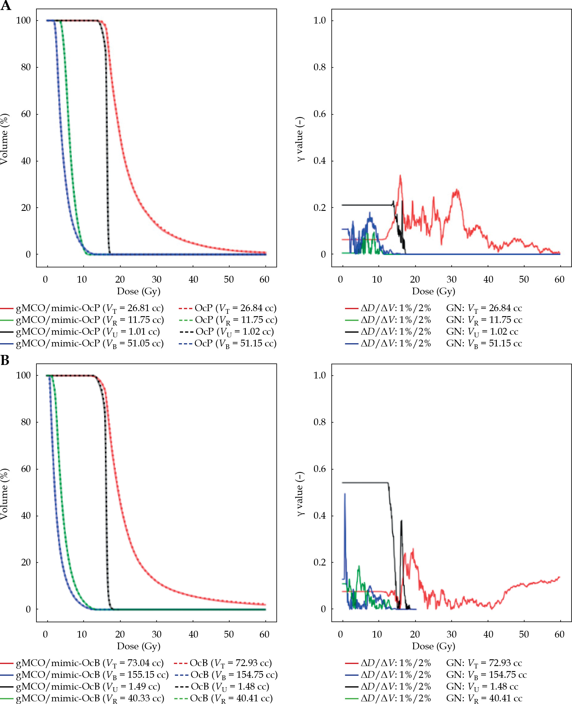
Table 4 summarizes the results of the 1D γ analysis of DVH curves between gMCO and OcP/OcB with the mimic parameters ON and OFF. As shown in Table 4, the γ index passed for all patients with gMCO with 1%/1% thresholds against OcP, and 1%/2% thresholds against OcB with the mimic parameters ON. While not included in Table 4, all the cases passed the γ analysis with 1%/4% thresholds with the mimic parameters OFF. Table 4 shows that failures of the γ analysis with the mimic parameters OFF for 1%/2% thresholds were mainly due to the target when compared with OcP, and the urethra compared with OcB.
Table 4
Results of γ index analysis of gMCO DVH curves with mimic parameters activated (ON) and deactivated (OFF) compared with OcP/OcB DVH curves (Ref.). Dose criterion was fixed at ΔD = 0.15 Gy (i.e., 1% of the prescribed dose). Volume criterion varied from 1% to 2% of structures’ volume. Numbers in row indicate number of patients, in which γ ≤ 1 for all bins
| Structure | Ref. | ΔD/ΔV | |||
|---|---|---|---|---|---|
| 1%/1% | 1%/2% | ||||
| Mimic | Mimic | ||||
| ON | OFF | ON | OFF | ||
| Target | OcP | 20 | 0 | 20 | 10 |
| OcB | 19 | 9 | 20 | 19 | |
| Urethra | OcP | 20 | 20 | 20 | 20 |
| OcB | 14 | 1 | 20 | 9 | |
| Bladder | OcP | 20 | 20 | 20 | 20 |
| OcB | 19 | 20 | 20 | 20 | |
| Rectum | OcP | 20 | 20 | 20 | 20 |
| OcB | 18 | 18 | 20 | 19 | |
| Total (/80) | OcP | 80 | 60 | 80 | 70 |
| OcB | 70 | 48 | 80 | 67 | |
Mitigating the impact of statistical uncertainties on DVH indices
By changing the seed of random generator in gMCO (100 times), a mean standard deviation (over 20 CT cases) of 0.05 cc in the bladder V75 and 0.03 cc in the rectum V75 was observed for 50,000 points (Figures S5 and S6 in Supplementary Material). The standard deviation was lower with the rectum V75 than the bladder V75 because the volume was smaller on average (Table 1) such that the point density was higher, thus leading to a lower statistical uncertainty. This was also observed for the US cases, where the bladder and rectum volumes were smaller compared with CT cases. As seen in Figure S5, the statistical uncertainty could be reduced with more random points [22], but with the consequence of increase memory consumption and computational time (e.g., average of 1.4 s with 50,000 points vs. 2.6 s with 100,000 points to compute 2,000 DVHs). To further mitigate statistical uncertainties, a statistical safety margin of 0.05 cc for the bladder and rectum volume indices was simulated for the CT cases (using V75 < 0.95 cc instead of V75 < 1.0 cc). When using this statistical safety margin of one SD with gMCO-GUI, a mean loss of 0.2% in the target coverage was observed compared with the plan with no margin. Using this safety margin would reduce the number of clinically relevant plans in gMCO plans bank (with target V100 ≥ 90% while meeting OARs criteria) by 4.4% on average, and would thus have limited impact considering that hundreds of plans were still available for plan navigation.
3D dose distributions
When comparing gMCO-GUI isodose lines (re-calculated from OcB exported RTDOSE as shown in Figure 4B) against OcB isodose lines (exported as RTSTRUCT as shown in Figure 4A), the 95% HD was below 0.01 mm for 75%, 100%, and 125% isodose lines, and was below 0.2 mm for 150% isodose line. Results of the spatial agreement of isodose lines obtained from gMCO 3D dose (e.g., Figure 4C) and OcP/OcB 3D dose (e.g., Figure 4B) are reported in Table 5. In most of the cases, the mean dice coefficient was over 0.98 (a value of 1 would mean that the isodose lines overlapped perfectly), and the mean 95% HD was below 0.4 mm. Based on the γ analysis (e.g., Figure 4D), the mean fraction of voxels with γ ≤ 1 when compared with OcP was 99.92% (range, 99.84-99.96%), and was 99.72% (range, 99.60-99.84%) when compared with OcB 3D dose distributions.
Fig. 4
Illustration of A) isodose lines in the middle slice for one random case as displayed in OcB. B) Isodose lines calculated with gMCO-GUI from OcB RTDOSE. C) Isodose lines calculated in gMCO-GUI from gMCO 3D dose. D) The γ map obtained when comparing gMCO 3D dose with OcB 3D dose. Colors are associated with isodose lines as follows: green – 75%, red – 100%, yellow – 125%, and cyan – 150%
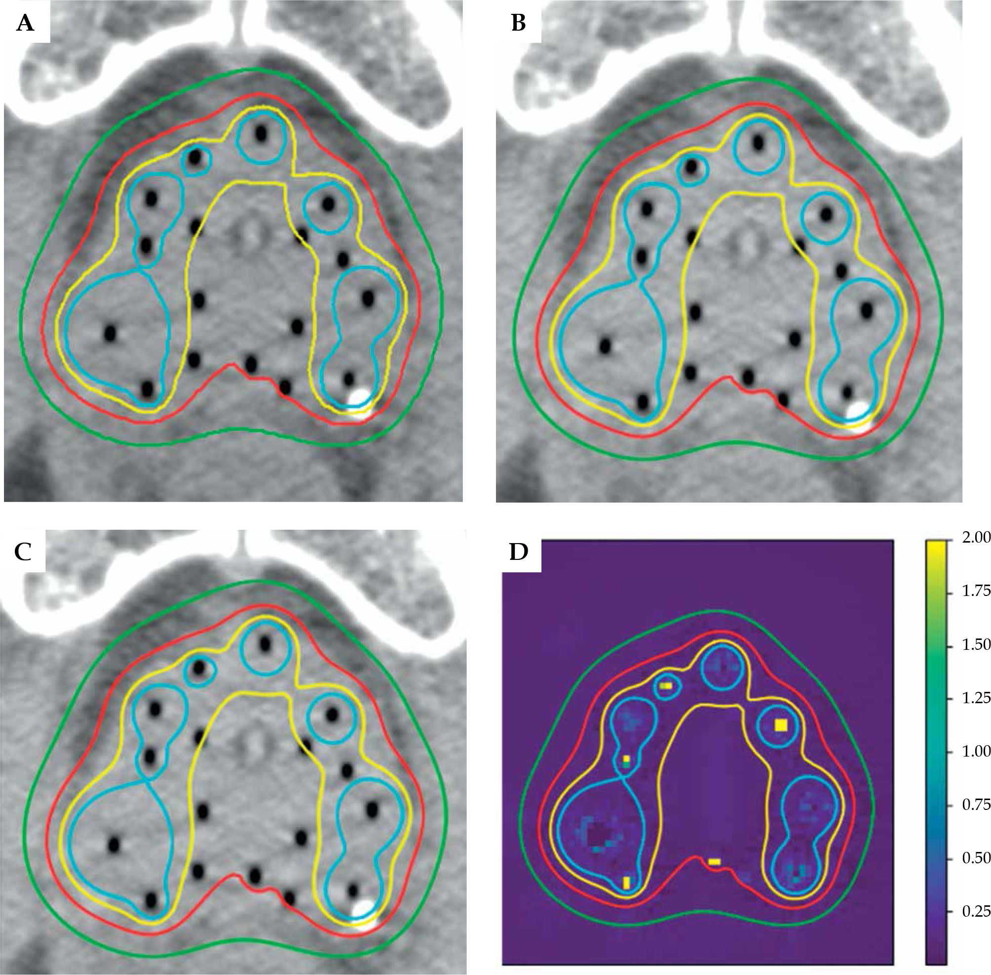
Table 5
Average dice coefficient and average 95th percentile undirected/bidirectional boundary Hausdorff distance (95% HD) between gMCO 3D dose and OcP/OcB 3D dose for different isodose levels (isodose lines were calculated using gMCO-GUI). Values in parenthesis indicate standard deviation around the average
Discussion
Regarding TG43 calculations, the calculated dose rates with gMCO were within –0.3% and 0.4% compared with the reference tabulated data (Tables 1-3 in the Supplementary Material). Hence, the calculated dose rates were well within the ±2% criteria established by the TG43 for TPS commissioning [23]. This suggests that the GPU-based TG43 implementation in gMCO is accurate.
Compared with the theoretical volumes (Table 3), the largest deviations were obtained with the sphere of 0.5 cm radius: –2.9% for gMCO, –3.3% for OcP, and –6.4% for OcB. Hence, gMCO and the two reference TPSs were outside the expected accuracy of 2% for the sphere with the smallest radius. For the cylinder with the smallest radius, gMCO and OcB calculated volumes were also outside of the 2% accuracy. Overall, gMCO calculated volumes were closer to the ground truth in 4/5 volumes compared with OcP/OcB. The agreement between gMCO structures’ volume and OcP/OcB structures’ volume was also within ±2% (Figure S2 in Supplementary Material).
When looking into dosimetric results (Figure 2), gMCO DVH indices values were within the ±2% tolerance compared to both TPSs (with a maximum deviation of 1.2%) with the mimic parameters ON. Larger differences observed in bladder V75 and rectum V75 (up to 0.13 cc or 13%) can be attributed in part to statistical uncertainties (Figures S5 and S6) from the fact that these are small volumes (0-1 cc) in large structures (50-250 cc; see Table 1). Nevertheless, the observed deviations (gMCO vs. OcP/OcB) are consistent with deviations obtained from the random sampling point simulations (Figure S6).
Left panels in Figure 3 show that gMCO DVH curves agreed with OcP or OcB DVH curves, suggesting that the agreement is valid for any DVH indices. This was further confirmed by the 1D γ analysis, in which 1%/2% threshold was needed to achieve an agreement for all patients between gMCO and OcP/OcB when comparing DVH curves (Table 4). While the differences met the desired accuracy of 2%, users must be aware that gMCO plans, with DVH indices close to institutional dosimetric criteria limit, may be violating these criteria after re-calculation in OcP/OcB (for final approval) due to numerical uncertainties (e.g., Figures S5 and S6). Nevertheless, a safety margin can easily be used with gMCO-GUI if needed to mitigate this effect as shown in the present study.
The rational to introduce mimic parameters in gMCO was because significant differences were initially observed in the tail of the target DVH curves (Figures S3 and S4 in Supplementary Material). With the mimic-OcP parameters OFF in gMCO, median differences of 1.5% (instead of –0.3%) in the target V150 as well as 2% (instead of –0.2%) in the target V200 were observed compared with OcP. While the proposed mimic-OcP parameters might not be strictly identical to TPS, and might not perfectly match the tails of the target DVH, the results indicate that the achieved accuracy is reasonable (within ±1% difference with OcP), such that it would have limited impact in the clinic. With the mimic-OcB parameters OFF in gMCO, median differences of –1.2% (instead of –0.3%) in the target V150 as well as –0.7% in the target V200 (instead of –0.1%) were observed with OcB. The 1D γ analysis further shows that deviations over 2% occurred with the mimic parameters OFF (Table 4). These observations suggest that there were more than 2% differences in the target V150 and target V200 between OcP and OcB when completing this study; this reinforce the importance of clearly stating the numerical parameters used in TPS to help the users understand what are the underlying impacts of such parameters that could influence decision-making process in the clinic [22].
Table 5 shows that the dice coefficient was over 0.98 for all isodose levels, which demonstrates the accuracy of spatial placement and shape of isodose lines in gMCO-GUI based on the 3D dose distribution (i.e., comparing the isodose lines in Figure 4C with 4B for all cases). In addition, a submillimeter accuracy (0.4 mm) was achieved based on 95% HD between gMCO and OcP/OcB isodose lines. The 95% HD was used in this study to mitigate the effect of very high-dose gradient regions (e.g., Figure 4).
Based on the 3D γ analysis using 1%/1 mm thresholds, the 3D dose distributions calculated by gMCO agreed with the ones calculated by OcP/OcB for more than 99% of the voxels (γ ≤ 1). But most of the evaluated voxels passed with γ ≤ 1 (Figure 4D), suggesting that the voxels that failed the criteria were close/inside the source (i.e., regions with high dose gradients), which was also observed in another study [34]. There are no clear guidelines on how to use the γ analysis in HDR brachytherapy, which have very high-dose gradient regions. Nevertheless, passing rate in external beam radiation therapy should be greater than 95% with 3%/2 mm threshold [35], while a preliminary study in brachytherapy suggested at least 98% with 2%/2 mm [34]. Given that the threshold used in this study was more stringent, it can be concluded that the γ analysis was successful for all cases and corroborated with the results obtained from the dice coefficient and Hausdorff analyses. Therefore, the 3D dose distributions in gMCO-GUI are both dosimetrically and spatially accurate (within the voxel size resolution of 1 mm).
The approach used in this study was to quantify the expected differences when using gMCO and gMCO-GUI combined with OcP or OcB in the clinic (Figure 1). However, this study did not conduct an in-depth characterization of how gMCO would perform against the ground truth for DVH curves and 3D dose distributions, since no such data were available. While only one plan per case were exported and validated against TPSs (thus hiding the other 1999 gMCO plans), it was not necessary to export more plans with the same patient for further validation. In fact, running gMCO with the same objective function parameters for all plans produced identical optimized dwell positions and dwell times, because of the deterministic nature of gL-BFGS optimizer [13]. Identical DVH curves and 3D dose distributions would therefore be created for all plans. Furthermore, since the trade-offs in gMCO are randomly generated and change from one patient to another, the exported plans’ ID (between 0 and 1,999) were random in the gMCO plans pool, thus mimicking how gMCO would be used in the clinic.
Finally, the end-to-end workflow depicted in Figure 1 was successfully tested for one case with OcP, including the transfer to flexitron. A bottleneck in the planning procedure was identified in the files’ transfer between OcP/OcB and gMCO, which would be resolved by integrating gMCO directly within the TPS. Nevertheless, our MCO workflow is readily available for clinical usage and the transfer to and validation by OcP/OcB maintain FDA-approved chain to the afterloader and patient treatment.
Conclusions
The proposed GPU-based MCO workflow was commissioned and validated against Oncentra Prostate and Oncentra Brachy, two widely used and clinically validated TPSs. TPS-specific numerical parameters regarding TG43 and DVH curves computations were introduced in gMCO to ensure minimal differences (less than 2%) with the two TPSs. Integrating gMCO and gMCO-GUI in a clinical TPS would facilitate the transition from single plan generated per optimization run to efficient GPU-based MCO optimizers in the clinic. This would allow fast and efficient navigation through patient-specific sets of Pareto-optimal plans in the clinic.