
Purpose
Prostate cancer is the most common cancer among men, and is the second-leading cause of cancer deaths in men in the United States [1]. Treatment methods include hormone therapy, chemotherapy, prostatectomy, and radiation therapy [2-4]. Hormone therapy reduces levels of hormones in the body to prevent them from allowing cancer cells to grow further. In chemotherapy, drugs are fed into the patient’s bloodstream to kill the tumor cells. Prostatectomy involves surgically removing all or parts of the prostate.
Radiation therapy uses high energy photons or charged particles to kill cancer cells. There are two main types of radiation therapy: external beam radiation therapy (EBRT) and brachytherapy. In EBRT, a medical linear accelerator produces high energy X-rays, and beams of radiation are focused on the prostate gland. In high-dose-rate (HDR) brachytherapy, radioactive source (e.g., iridium-192 [192Ir]) is temporarily placed in planned locations in the prostate for irradiating target volume. While, in low-dose-rate (LDR) brachytherapy, small radioactive seeds are implanted permanently into the patient’s prostate in order to deliver radiation directly to the gland while minimizing damage caused by the radiation dose received by nearby healthy tissue. These radioactive sources are generally iodine-125 (125I), palladium-103 (103Pd), or cesium-131 (131Cs) seeds. Number of seeds is determined by a treatment planning system, and implanted seeds remain permanently in the prostate and radioactive seeds decay to a background level after a period of time.
In the operating room, radioactive seeds are placed into the prostate gland using hollow needles with ultrasound image guidance. Handling of radioactive seeds is subject to federal regulations in the United States for radiation safety, and a radiation survey has to be performed at the end of every procedure. One of the important tasks is to make sure the number of seeds implanted in the patient are correct according to the treatment plan. To the best of our knowledge, there are no existing methods of auto-detecting of implanted seeds on fluoroscopy images, except counting with naked eyes. In current clinical practice, the correctness is inferred by counting the leftover seeds and assuming that the rest of seeds are placed inside the patient’s prostate gland. However, there is no actual counting of the number of seeds shown on the fluoroscopy. It is to note that ultrasound image is not sufficient to detect all the seeds, and the only other commonly available imaging modality in operating room (OR) is C-ARM fluoroscopy. In rare situations, seeds could be sucked into the withdrawing needle or block the opening of the needle, and seeds could drop out of the patient or be carried away in the patient’s body with bloodstream. In these scenarios, to count the number of seeds displayed in the fluoroscopy that are actually in the patient’s prostate, is a definitive verification. In addition, as a good practice, taking a final fluoroscopy at the end of a procedure to ensure that all seeds are inside the patient can rule out the assumption from inference by counting only the leftover seeds. At the end of a surgery, a radiation detector is used to perform a survey of the surrounding area to ensure that there are no radiative seeds left outside the patient. In an operating room, where the goal is to accomplish tasks as quickly and safely as possible, manually counting every seed while under pressure would consume too much time, and is difficult due to large number of seeds (usually more than 50) implanted and their diminutive size.
In this work, we proposed the use of region-based convolution neural networks (R-CNN) [5] approach for automatic seed detection in a fluoroscopy image. R-CNN has a number of useful applications, primarily in object detection. We investigated the efficacy of using R-CNN for seed detection to reduce the time needed to acquire an accurate count of the number of seeds implanted in the patient.
Material and methods
Dataset and pre-processing
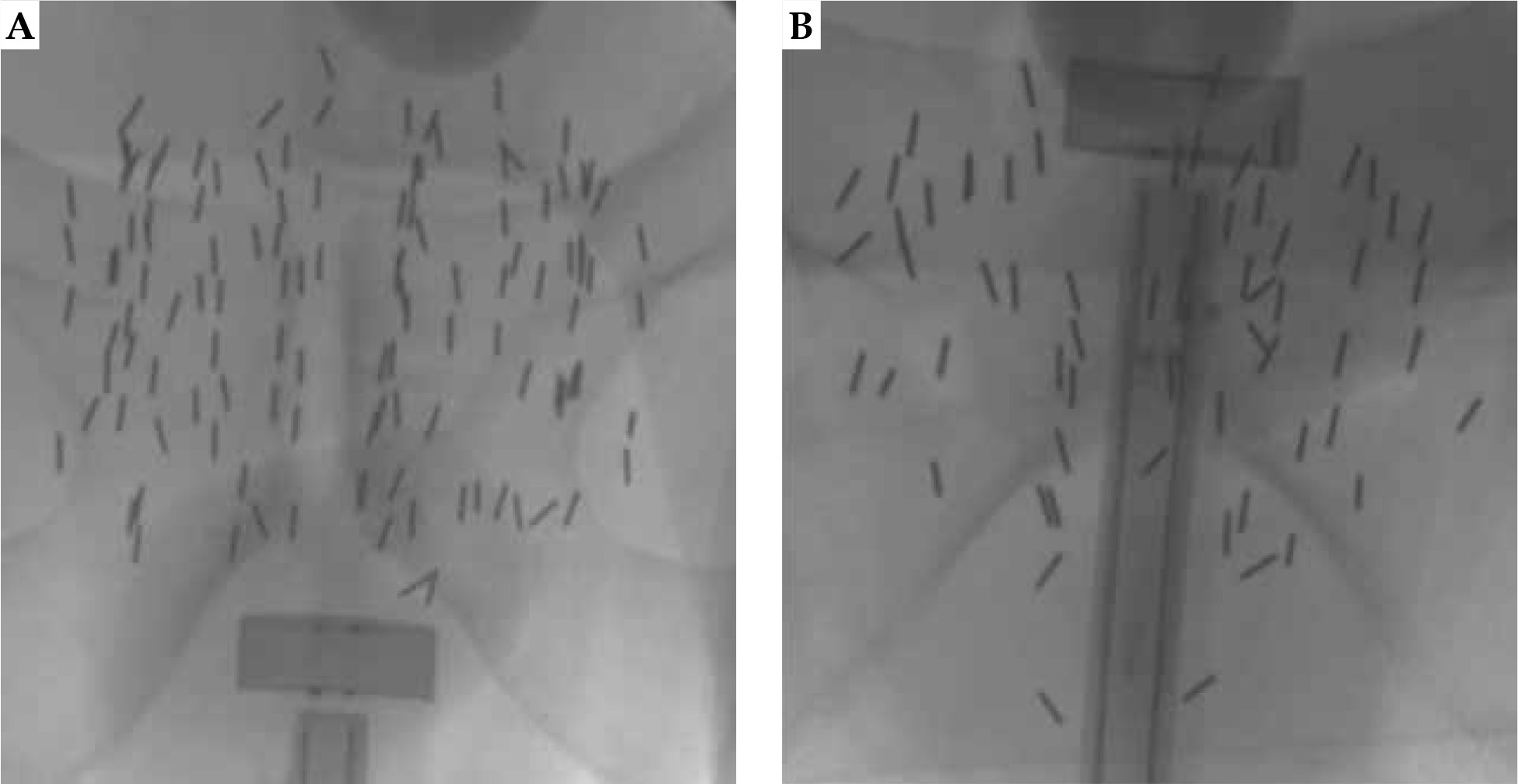
Forty-eight fluoroscopy images of patients who underwent prostate seed implant (PSI) from January 2014 to March 2021 for this study (STUDY20210259) were investigated, after our University Hospitals Institutional Review Boards (UH IRB) approval. Radioactive seeds used in the patients were 125I (AgX100) produced by Theragencis Corporation, Buford, GA. An 125I seed consists of a cylindrical titanium encapsulation, which contains a silver rod substrated by 125I, and physical dimension of the seed is 4.5 mm in length and 0.8 mm in diameter. Fluoroscopy images were acquired with a GE OEC C-ARM medical system. Kilo-voltage peak of X-ray tube ranged from 81 kV to 105 kV, and exposure time was from 350 msec to 608 msec, with a radiation setting of high-dose exposure. Dimensions of the image in pixels were 980 × 980. During the seed implant procedure in the operating room, a Foley catheter was placed in the patient’s bladder to drain urine, and diluted contrast was injected into a Foley balloon. The Foley is then retracted to the bladder neck. A radiation oncologist then examined the patient’s prostate using a transrectal ultrasound (TRUS) probe to localize the prostate apex and base, and then TRUS images were acquired. A treatment plan was generated based on ultrasound images. A device, called ‘Mick® applicator’ (Mick Radio-Nuclear Instruments, Inc.) was applied to deliver the seeds into the prostate using a template grid. Fluoroscopy images were taken to verify locations of the implanted seeds, and to ensure no seeds were in the bladder. The other purpose of the fluoroscopy image was to verify the number of implanted seeds by actually counting the seeds in the image. Two examples of the fluoroscopy image are shown in Figure 1. The Foley balloon in the bladder, TRUS probe at the apex (Figure 1A), and the base (Figure 1B) of the prostate from two different cases with the implanted seeds can be clearly seen.
Four pre-processing steps were used to prepare for the training data. First, we manually contoured each seed with a brush tool using MIM software v. 7.0.6 (Cleveland, OH, USA). Initially, we tried to use an automatic contour tool, which was based on pixel intensity provided in MIM software, but it did not meet our expectation. Therefore, we contoured each individual seed manually, and the number of contoured seeds was the ground truth of counting. With the contour data, we were able to find bounding box for each seed, represented by (xmin, ymin), (xmax, ymax), which served as the ground truth bounding box. The second step was normalization for the seed size. We observed that the seeds on different images had different sizes, because the magnification factor for each case due to the distance of X-ray tube to the patient surface was different. The difference also originated from the orientation of the seeds relative to X-ray direction inside the patient. Since no distance information was provided in radiographic fluoroscopy (RF) DICOM tags, we could not derive the magnification factor directly. Therefore, a simple method was used to understand the factor. We decided on an upright seed from each image, and randomly chose one of them as a reference seed. Bounding box of the reference seed was applied to normalize all other images by matching the dimension of the chosen seed to that of the reference seed. Image resolution was kept as 1 : 1 (no units since they were ratios). Then, we cropped each image manually into a rectangle region, which had the implanted seeds. The cropped images had dimensions ranging from 300 to 800 pixels for both (I, J) directions. Finally, since the input to the network (faster R-CNN) required images in RGB color space (3 data channels), we needed to convert the fluoroscopy image into PNG format. Mean (x) and standard deviation (δ) of the image pixel value were calculated first. Lower and upper boundaries of a rescale table was set as (x–3δ, x+3δ). The rescale table was used to map the image pixel value to a value between 0 and 255 (data type of unsigned char). Rescaled grayscale values were applied for each color channel, that is, the values of red, green, and blue channel were the same. Therefore, the results were not dependent on color channels, and original data values were preserved. The final input image data to the network was in PNG format, and contained no patient identification information.
Learning network
Faster R-CNN [5] has been successfully applied to a number of tasks for object detection and localization. It is one of the accurate deep learning models that predicts both bounding boxes and class scores for objects in an image. In faster R-CNN, convolutional feature maps are first extracted from a fully convolutional network and then, a separate network is used to predict the region proposals. It eliminates the selective search and allows the network to learn the regional proposals, which makes it faster. In our work, we used an implementation of this network in an open source machine learning library (PyTorch) [6]. We started with an example from a tutorial of this library (TorchVision Objection Detection) and adapted the code to our project.
A transfer learning technique on our datasets of fluoroscopy images was employed to train a CNN for automatically detecting the implanted seeds in the image [7, 8]. Transfer learning is a machine learning method that uses a pre-trained model based on a large dataset, and applies the model to a user-specified task. The recognized features that were obtained by a pre-trained model can facilitate the training process for user-provided data. In our case, we used a pre-trained faster R-CNN model on COCO object [9] localization dataset with a ResNet-50 backbone, and fine-tuned it for training on our image dataset. ResNet-50 [10] consists of four convolution stages, with a total of 50 layers. A pre-trained model can be obtained from TorchVision in the PyTorch library with a function call (fasterrcnn_resnet50_fpn).
To evaluate the performance of our model, the leave-one-out cross-validation (LOOCV) procedure [11] was used. LOOCV is a k-fold cross-validation method, where k equals N, and N is the number of training data points in the dataset. K-fold cross-validation can be applied to estimate the performance of a machine learning algorithm for predictions on data not used during the training of the model. The parameter “k” is the number of subsets that a dataset is split into. In the training, one subset is held out as a test set, so that the other k-1 subsets are used as training datasets, and each subset in the k-fold will be used as a test set. The model performance was evaluated using a summary statistics from the results of the hold-out training datasets. In LOOCV, each case is used as the test data, and therefore a model is generated and evaluated for each case. The procedure is computationally expensive; however, it is appropriate for a small dataset, such as 48 cases in the present study.
Performance metrics
The performance of algorithm was measured using the mean average precision and recall at different intersection over union (IoU) thresholds [12]. The detected box of a seed was compared with the ground truth bounding box by calculating IoU, which was defined as:
where A is the predicted bounding box, and B is the ground truth bounding box. It specified the amount of overlap between the predicted and ground truth bounding boxes, ranging from 0 (no overlap between the two sets) to 1 (completely overlapped). To define a hit-or-miss detection of an object, an overlap criterion was used. For example, for a given threshold of 0.5, a predicted bounding box was considered a detected seed, deemed as true positive (TP), if the intersection over union with the ground truth bounding box was greater than 0.5; otherwise, no seed was considered detected, and it was deemed false positive (FP). If there was no detection of a true bounding box, it was false negative (FN). At a given threshold IoU value t, the precision and recall were calculated as:
The precision is the ratio of the number of correctly predicted seeds (TP), divided by the total number of model bounding box predictions (whether correctly predicted or no), and the recall is the ratio of the number of correctly predicted seeds (TP), divided by the total number of correctly predicted seeds plus the number of true seeds not detected by the algorithm. The mean average precision (mAP) and recall (mAR) for one fluoroscopy image were calculated as the mean of the above precision and recall values at each IoU threshold, where t is the threshold IoU value, and T is the total number of the defined threshold values:
Additionally, F1-score was calculated according to the following formula:
We employed a Python application programming interface library called ‘pycocotools’ for the calculation of the above-mentioned metrics. The confidence score of each seed detected by the model in the image was set to 0.4, i.e., all of the predicted bounding boxes with a confident score above 0.4 were considered as positive boxes.
Results
The learning algorithm based on leave-one-out cross-validation was evaluated, and the results for each test leave-one-out dataset were reported. The training and testing were carried out using a CUDA-enabled graphical card (TITAN XP), with 12 GB display memory. We used the following parameter settings of PyTorch implemented faster R-CNN for this project: number of epoch = 50, number of classes = 2 (background and radioactive seeds), initial learning rate = 0.005, decay rate = 5.e-4, momentum = 0.9, number of box detections per image = 200 (assuming that the number of implanted seeds did not exceed 200), weights on the bounding box = (1, 1, 1, 1), and for other options, such as parameters in the region proposal network, the default settings in the PyTorch library was applied.
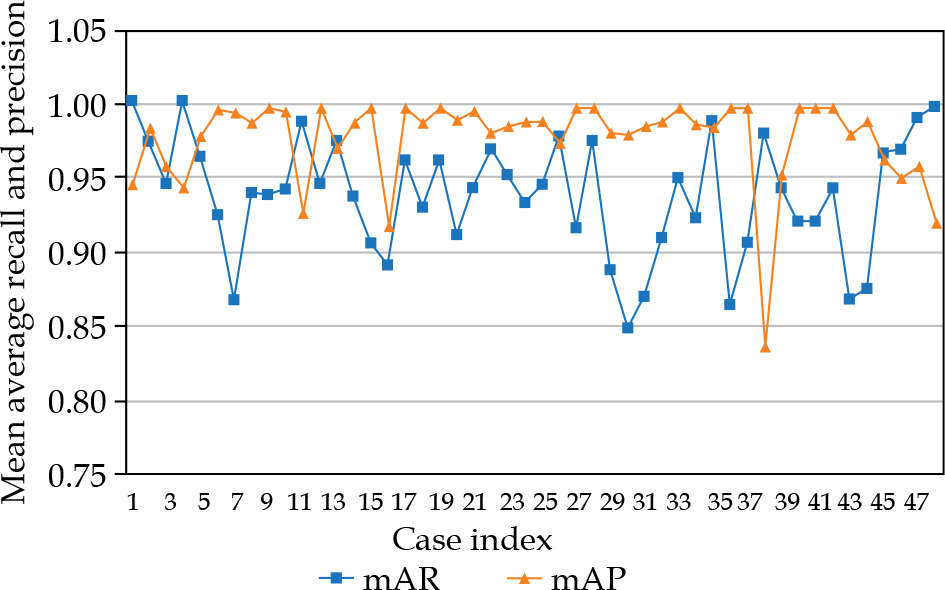
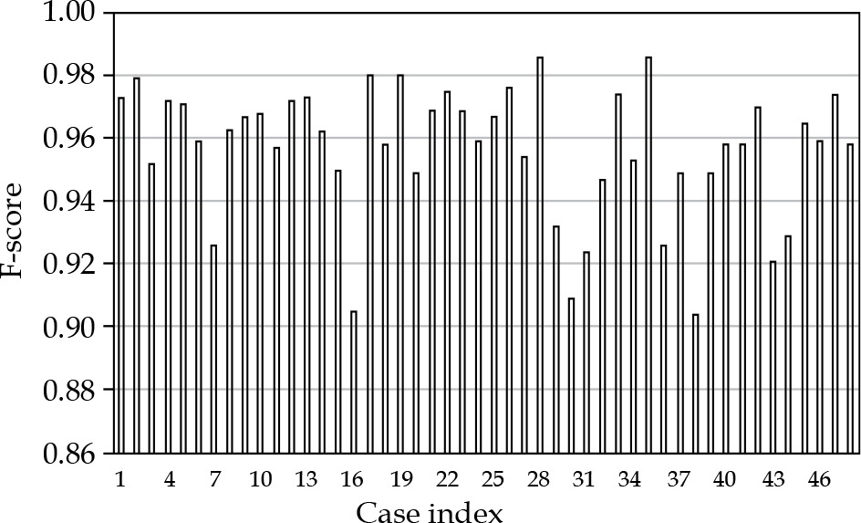
Figure 2 shows the detection results of mAP and mAR for each case. All cases, except one, had mAP values > 0.9. There were 8 cases (16.7%) that had mAR values < 0.9, but greater than 0.85, and 40 cases (83.3%) were with mAR > 0.9. F1-scores for all the cases were greater than 0.9, and are shown in Figure 3. The averaged results were 0.979 (SD: 0.03, min: 0.839, max: 1.0), 0.937 (SD: 0.04, min: 0.847, max: 1.0), and 0.957 (SD: 0.02, min: 0.904, max: 0.986) for mAP, mAR, and F1-score, respectively. Note that precision in the context of seed detection referred to the ratio of the number of the detected true seeds (true positive) to the total number of the seed predictions, which may include falsely identified seeds (false positive), while recall referred to the ratio of the number of the detected true seeds (true positive) to the total number of the true seeds (some of these true seed may not be detected by the algorithm (false negative)). The mean averaged precision and recall were calculated as the mean of precision and recall at all pre-defined thresholds (IoU) that were applied for the algorithm to show if a prediction was a true seed or not. Our algorithm provided 97.9% accuracy to predict a seed, and 6.3% chance to fail to detect a real seed. To investigate the accuracy of naked-eye counting, four clinicians were requested to carry out the task. A stopwatch was used to record the counting time. There were 4,114 seeds of all 48 cases, and this number was from the seed contours and referred to as the ground truth. The counting error from the four clinicians was within 0.25% (a variation about 10 seeds in the counting existed among the four clinicians due to different interpretation of overlapped seeds). However, the time spent to count one seed was about 1 second, while it took the algorithm less than 1 second to count all seeds in one image.
Fig. 2
Results of mean average recall (mAR) and precision (mAP) for all cases using leave-one-out cross-validation
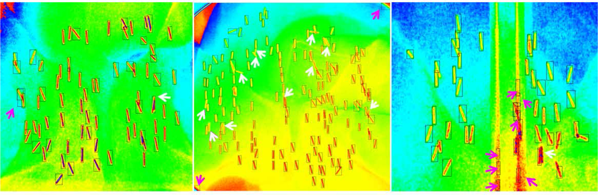
To better explain the results, we demonstrated three cases (Figure 4), which corresponded to case #35, #30, and #38 in Figure 3. For case #35 (mAP, 0.986, mAR, 0.986), all but two of the implanted seeds were correctly identified by the algorithm: one was false positive (purple arrow), and one was false negative (white arrow). In case #30, most of the seeds were correctly identified; however, there were some overlapping seeds unaccounted, as shown by white arrows (false negative) and two corner residues from cutting of the edge of the field of view that were mistakenly accounted as seeds (false positive). For this case, the mAP was high (0.987) but the mAR was low (0.868). In contrast, for case #38, the mAP was low (0.839), while the mAR was high (0.979). There were seven false positive seeds resulting from misinterpretation by the algorithm due to the edge of TRUS probe. One false negative seed almost overlapped with the other, and was not accounted for.
Discussion
We could see that the method could accurately detect well-separated seeds; however, several limitations were observed in the study. First, as we know, small object detection has been a challenging task in the field of artificial intelligence. Part of the challenge is due to the limited amount of information representing small crowded objects and overlapping with other objects [13-16]. This was the case in our work, as the seeds in fluoroscopy images were small objects and often overlapped partially with other seeds, forming a cluster of seeds. Misinterpretations of overlapping seeds or a cluster of seeds lead to a decrease in accuracy due to false negative detections. The issue of seed overlapping could be alleviated by taking multiple fluoroscopy images at different acquisition angles. However, in a time-constrained operating room, the position of C-ARM device is not usually moved after initial setup. Actually, it is the anterior-to-posterior direction, at which a fluoroscopy image is taken in clinical practice. Moreover, the overlapped seeds can still be seen in the image taken at a different acquisition angle. Besides the challenge of detecting overlapped seeds, the second difficulty come from distinguishing small non-seed artificial objects and the edges of the TRUS probe from multiple seeds. There are cases that the probe is inside the patient while the fluoroscopy image is taken, for example, when the physicians want to know the location of the probe relative to the patient’s anatomy. The probe in the fluoroscopy image is shown as two parallel lines. Non-uniformity of the image intensity of the lines can lead the algorithm to falsely identify the probe edges as multiple seeds. The third limitation may come from the pre-trained model parameters in the library (PyTorch). The pre-trained model is based on training of COCO and PASCAL VOC [17] datasets, and these datasets contain more medium or big objects than small objects, which may cause an imbalance data of different sizes, and therefore result in potentially biasing the detection model to focus more on large objects rather than small objects, as encountered in our work.
Techniques have been seen in the literature to improve the accuracy of small object detection using R-CNN [5]. One commonly used technique is the augmentation. In this method, small objects in the images are oversampled and augmented by copy-pasting many times. Each seed in our study usually occupied several tens of pixels in the image. Increasing the image resolution can increase the number of pixels for each seed; however, it increases the computational time. It is uncertain if the method could improve the accuracy of detecting the overlapping or clustered seeds, as all the seed dimensions are proportionally increased. The other ways of artificially augmenting dataset include rotation of images with different angles and copy-pasting small objects to different locations in the image. Specific to our project, the augmentation could be carried out in our future work by copying the instance of overlapping seeds, rotating by different angles, and re-locating to other locations. However, the simple way without staining the original image is to increase the size of training dataset. There were only 48 cases of 125I PSI used in the current study. In future work, we will include more cases and build a database of 103Pd PSI. With a larger dataset, more accurate results would be produced, which could better validate our results. The other technique that has also been used to improve the accuracy of small object detection is using different networks (ResNet-101-FPN and VGG-16) for backbones and feature extractors. Our future work will further investigate this approach.
With limited datasets for training and intricate difficulties from seed overlapping, it is challenging to eliminate the false negative or the false positive detections for the implanted seeds in the fluoroscopy images. By including more datasets for training in the future, it is possible to achieve higher accuracy in seed counting. In clinical PSI procedures, since the seeds are radioactive, every seed must be counted according to regulation’s requirement for radiation safety. Given the complex variation in generating the fluoroscopy image for each individual patient, it may be impractical for an artificial intelligence numerical model to produce 100% accuracy for all situations. Therefore, building a human-assisted system is necessary. As we can imagine, counting the number of implanted seeds (50-100 seeds) by naked eyes is very time-consuming and error-prone. A human-assisted system can make the counting much faster and easier in the proposed process as the following. The implanted seeds are initially identified by a deep learning model, and a table is shown up to list the identified bounding boxes that have low confidence scores. Detections with low confidence scores are potentially false negative or false positive. Clinicians go through these bounding boxes with a user interface to identify real seeds. A deployment of the model to certified mobile cell phones could make the counting process further easier by taking the image from a C-ARM screen directly with a phone. We consider building such a system in the future.
Conclusions
In the present study, a faster R-CNN deep learning library was applied to automatically detect implanted radioactive seeds in the fluoroscopy images from PSI procedure. The method achieved a good accuracy, with an averaged mean precision of 0.979, averaged mean recall of 0.937, and F1-score of 0.957. The achieved accuracy provides the potential for the application of the method to count the number of seeds implanted in patients in the operating room faster and easier.